
DEEP LEARNING OF MICROSTRUCTURES
by
Amir Abbas Kazemzadeh Farizhandi
A dissertation
submitted in partial fulfillment
of the requirements for the degree of
Doctor of Philosophy in Computing, Data Science
Boise State University
December 2022
© 2022
Amir Abbas Kazemzadeh Farizhandi
ALL RIGHTS RESERVED
BOISE STATE UNIVERSITY GRADUATE COLLEGE
DEFENSE COMMITTEE AND FINAL READING APPROVALS
of the dissertation submitted by
Amir Abbas Kazemzadeh Farizhandi
Dissertation Title: Deep Learning of Microstructures
Date of Final Oral Examination: 19 October 2022
The following individuals read and discussed the dissertation submitted by student Amir Abbas Kazemzadeh Farizhandi, and they evaluated their presentation and response to questions during the final oral examination. They found that the student passed the final oral examination.
Mahmood Mamivand, Ph.D. Chair, Supervisory Committee
Edoardo Serra, Ph.D. Member, Supervisory Committee
Eric Jankowski, Ph.D. Member, Supervisory Committee
The final reading approval of the dissertation was granted by Mahmood Mamivand, Ph.D., Chair of the Supervisory Committee. The dissertation was approved by the Graduate College.
DEDICATION
I dedicate my dissertation work to my family. A special feeling of gratitude to my loving wife and parents, whose words of encouragement and push for tenacity ring in my ears.
ACKNOWLEDGMENTS
I would like to express my sincere thanks and appreciation to my supervisor, Dr. Mahmood Mamivand, for his invaluable guidance, support, and suggestions. His knowledge, suggestions, and discussions help me to become a capable researcher. His encouragement also helped me to overcome the difficulties encountered in my research. I would also like to thank Dr. Edoardo Serra and Dr. Eric Jankowski for serving as my committee members. I am very grateful to my lovely wife, who always supports me. Last but not least, I want to thank my parents, brother, and sister in Iran for their constant love and encouragement.
ABSTRACT
The internal structure of materials also called the microstructure plays a critical role in the properties and performance of materials. The chemical element composition is one of the most critical factors in changing the structure of materials. However, the chemical composition alone is not the determining factor, and a change in the production process can also significantly alter the materials’ structure. Therefore, many efforts have been made to discover and improve production methods to optimize the functional properties of materials.
The most critical challenge in finding materials with enhanced properties is to understand and define the salient features of the structure of materials that have the most significant impact on the desired property. In other words, by process, structure, and property (PSP) linkages, the effect of changing process variables on material structure and, consequently, the property can be examined and used as a powerful tool in material design with desirable characteristics. In particular, forward PSP linkages construction has received considerable attention thanks to the sophisticated physics-based models. Recently, machine learning (ML), and data science have also been used as powerful tools to find PSP linkages in materials science. One key advantage of the ML-based models is their ability to construct both forward and inverse PSP linkages. Early ML models in materials science were primarily focused on process-property linkages construction. Recently, more micro structures are included in the materials design ML models. However, the inverse design of micro structures, i.e., the prediction of process and chemistry from a micro structure morphology image have received limited attention. This is a critical knowledge gap to address specifically for the problems that the ideal micro structure or morphology with the specific chemistry associated with the morphological domains are known, but the chemistry and processing which would lead to that ideal morphology are unknown.
In this study, first, we propose a framework based on a deep learning approach that enables us to predict the chemistry and processing history just by reading the morphological distribution of one element. As a case study, we used a dataset from
spinodal decomposition simulation of Fe-Cr-Co alloy created by the phase-field method. The mixed dataset, which includes both images, i.e., the morphology of Fe distribution, and continuous data, i.e., the Fe minimum and maximum concentration in the micro structures, are used as input data, and the spinodal temperature and initial chemical composition are utilized as the output data to train the proposed deep neural network. The proposed convolutional layers were compared with pretrained EfficientNet convolutional layers as transfer learning in micro structure feature extraction. The results show that the trained shallow network is effective for chemistry prediction. However, accurate prediction of processing temperature requires more complex feature extraction from the morphology of the micro structure. We bench marked the model predictive accuracy for real alloy systems with a Fe-Cr-Co transmission electron microscopy micro graph. The predicted chemistry and heat treatment temperature were in good agreement with the ground truth. The treatment time was considered to be constant in the first study. In the second work, we propose a fused-data deep learning framework that can predict the heat treatment time as well as temperature and initial chemical compositions by reading the morphology of Fe distribution and its concentration. The results show that the trained deep neural network has the highest accuracy for chemistry and then time and temperature. We identified two scenarios for inaccurate predictions; 1) There are several paths for an identical micro structure, and 2) Micro structures reach steady-state morphologies after a long time of aging. The error analysis shows that most of the wrong predictions are not wrong, but the other right answers. We validated the model successfully with an experimental Fe-Cr-Co transmission electron microscopy micro graph.
Finally, since the data generation by simulation is computationally expensive, we propose a quick and accurate Predictive Recurrent Neural Network (PredRNN) model for the micro structure evolution prediction. Essentially, micro structure evolution prediction is a spatiotemporal sequence prediction problem, where the prediction of material microstructure is difficult due to different process histories and chemistry. As a case study, we used a dataset from spinodal decomposition simulation of Fe-Cr-Co alloy created by the phase-field method for training and predicting future microstructures by previous observations. The results show that the trained network is capable of efficient prediction of microstructure evolution.
TABLE OF CONTENTS
DEDICATION …………………………………………………………………………………………………
ACKNOWLEDGMENTS …………………………………………………………………………………..
ABSTRACT …………………………………………………………………………………………………….
LIST OF TABLES …………………………………………………………………………………………..
LIST OF FIGURES ………………………………………………………………………………………..
LIST OF ABBREVIATIONS …………………………………………………………………………..
CHAPTER ONE: INTRODUCTION ……………………………………………………………………
Process-Structure-Property Linkages …………………………………………………………..
Materials Microstructure Evolution Prediction ……………………………………………..
Dissertation Structure ……………………………………………………………………………..
CHAPTER TWO: METHOD …………………………………………………………………………….
Phase Field Method ………………………………………………………………………………..
Dataset Generation …………………………………………………………………………………
Dataset Generation for Steady State Case Study ……………………………….
Dataset Generation for Unsteady State Case Study ……………………………
Dataset Generation for Microstructure Evolution Case Study………………
Deep Learning Methodology ……………………………………………………………………
Fully-Connected Layers………………………………………………………………..
Convolutional Neural Networks (CNN) …………………………………………..
Proposed Model for Steady State Case Study ……………………………………………..
Proposed Model for Unsteady State Case Study ………………………………………….
Proposed Model for Microstructure Evolution Prediction …………………………….
Measure the Similarity Between Images ……………………………………………………
CHAPTER THREE: DEEP LEARNING APPROACH FOR CHEMISTRY AND PROCESSING HISTORY PREDICTION FROM MATERIALS MICROSTRUCTURE
…………………………………………………………………………………………………………………….
Phase-Field Modeling and Dataset Generation ……………………………………………
Convolutional Layers for Feature Extraction ………………………………………………
Temperature and Chemical Compositions Prediction …………………………………..
Validation of The Proposed Model with The Experimental Data ……………………
Conclusion …………………………………………………………………………………………..
Data availability ……………………………………………………………………………………
CHAPTER FOUR: PROCESSING TIME, TEMPERATURE, AND INITIAL CHEMICAL COMPOSITION PREDICTION FROM MATERIALS MICROSTRUCTURE BY DEEP NETWORK FOR MULTIPLE INPUTS AND FUSED
DATA ……………………………………………………………………………………………………………
Phase-Field Modeling and Dataset Generation ……………………………………………
Deep Network Training ………………………………………………………………………….
Model Performance Analysis …………………………………………………………………..
Validation of The Proposed Model with the Experimental Data …………………….
Conclusion …………………………………………………………………………………………..
Data availability ……………………………………………………………………………………
CHAPTER FIVE: SPATIOTEMPORAL PREDICTION OF MICROSTRUCTURE EVOLUTION WITH PREDICTIVE RECURRENT NEURAL NETWORK …………….
Phase-Field Modeling for Microstructure Sequences Generation …………………..
Microstructure Evolution Prediction by PredRNN ……………………………………….
Trained Model Performance on The Microstructure Evolution Prediction During Time ……………………………………………………………………………………………………
Trained Model Inference Performance in Future Microstructures Prediction ……
Conclusion ……………………………………………………………………………………………
Data availability …………………………………………………………………………………….
CONCLUSION AND FUTURE WORKS ……………………………………………………………
Future Works ………………………………………………………………………………………..
REFERENCES ………………………………………………………………………………………………..
LIST OF TABLES
Table 2.1 Phase-field model input parameters [100, 102, 103] ………………………….
Table 2.2 Simulation variables and their range of values for database generation of steady state case study. …………………………………………………………………
Table 2.3 Simulation variables and their range of values for database generation of unsteady state case study. ……………………………………………………………..
Table 2.4 Parameters selected for model specification, compilation, and cross validation. ………………………………………………………………………………….
Table 3.1 R-squared and MSE of model predictions for training and testing dataset when different layers of EfficientNet-B6 are used for microstructures’ feature extraction. ……………………………………………………………………….
Table 3.2 R-squared and MSE of model predictions for training and testing dataset when different layers of EfficientNet-B7 are used for microstructures’ feature extraction. ……………………………………………………………………….
Table 4.1 Performance of network with different in-house CNNs. …………………….
Table 4.2 R-squared and MSE of model predictions for training and testing datasets when different layers of EfficientNet-B7 were used for microstructures’ feature extraction. ……………………………………………………………………….
LIST OF FIGURES
Figure 1.1 Schematic of materials design workflow by forward and inverse design using PSP linkages. ……………………………………………………………………….
Figure 2.1 Schematic of a typical convolutional neural network. ………………………..
Figure 2.2 The flowchart of the developed model for chemistry and processing history prediction from microstructure images (FC: fully-connected layer) …………………………………………………………………………………………………
Figure 2.3 The flowchart of the developed model for chemistry and processing history prediction from microstructure images (FC: fully-connected layer)…………………………………………………………………………………………………
Figure 2.4 The flowchart of the developed model for chemistry, time, and temperature prediction from microstructure images (FC: fully-connected layer) …………………………………………………………………………………………
Figure 2.5 Left: the main architecture of PredRNN, in which the orange arrows denote the state transition paths of Ml t, namely the spatiotemporal memory flow. Right: the ST-LSTM unit with twisted memory states serves as the building block of the proposed PredRNN, where the orange circles denote the unique structures compared with ConvLSTM (the figure was adopted from the original study [157]). ……………………………………………………….
Figure 2.6 (a) A real two-phase microstructure, (b) and (c) a simple checkerboard microstructure for presenting X_uv and two-point correlation (white color is phase 1 and black color is phase 2) ………………………………………………
Figure 3.1 Fe-Cr-Co alloys microstructure generated by the phase-field method for:a) Fe-20%, Cr-40%, Co-40% at 873K, b) Fe-20%, Cr-40%, Co-40% at963K, c) Fe-25%, Cr-30%, Co-45% at 933K. (Composition are in atomic percent). …………………………………………………………………………………….
Figure 3.2 A sample workflow of dataset construction………………………………………
Figure 3.3 Sample response maps in developed CNN for 2D microstructure morphology inputs. The response map of the first four filters of three
convolutional layers is illustrated for three input images. The layer
numbers are presented at the top of the images. ………………………………..
Figure 3.4 Sample response maps in EfficientNetB7 for 2D microstructure morphology inputs. The response map of the first four filters of some convolutional layers is illustrated for three input images. The layer numbers are presented at the top of the images. ………………………………..
Figure 3.5 Sample response maps in EfficientNetB6 with 2D microstructure inputs. The response map of the first four filters of some convolutional layers is illustrated for three input images. The layer number is presented at the top of the figure. ………………………………………………………………………………
Figure 3.6 The architecture of the proposed model (input image size is 224 × 224 pixels). ………………………………………………………………………………………
Figure 3.7 a) Training and validation loss per each epoch, b) prediction of temperature and chemical compositions for a test dataset, and c) the parity plots of temperature and chemical compositions for the testing dataset from the proposed model when proposed CNN are used for microstructures’ feature extraction (input image size is 224 × 224 pixels)
………………………………………………………………………………………………..
Figure 3.8 a) Training and validation loss per each epoch, b) prediction of temperature and chemical compositions for a random test dataset, and c) the parity plots of temperature and chemical compositions for the testing dataset from the proposed model when first 806 layers of EfficientNetB7 are used for microstructures’ feature extraction (The size of the input images are 224 × 224 pixels) …………………………………………………………
Figure 3.8 a) Training and validation loss per each epoch, b) prediction of temperature and chemical compositions for a test dataset, and c) the parity plots of temperature and chemical compositions for the testing dataset from the proposed model when proposed CNN are used for micro structures’ feature extraction (input image size is 224 × 224 pixels)
………………………………………………………………………………………………..
Figure 3.10 Prediction of chemistry and processing temperature for an experimental TEM image adopted from Okada et al. [182]. The original image was cropped to be in the desired size of 224 × 224 pixels. ………………………..
Figure 4.1 The phase-field method generates Fe-Cr-Co alloy microstructures (Compositions are in atomic percent). …………………………………………….
Figure 4.2 A sample workflow of dataset construction. …………………………………….
Figure 4.3 Sample response maps in EfficientNetB7 with 2D microstructure inputs. The response map of the first four filters of some convolutional layers is illustrated for four input images. The layer number is presented at the top
of the figure. ……………………………………………………………………………….
Figure 4.4 The architecture of the proposed model (input image size is 224 × 224 pixels). ………………………………………………………………………………………
Figure 4.5 Error distribution for the testing dataset from the proposed model when the first 286 layers of EfficientNetB7 are used for microstructures’ feature extraction (The size of the input images is 224 × 224 pixels) ………………
Figure 4.6 a) Training and validation loss per each epoch, b) prediction of time, temperature, and chemical compositions for a random test dataset, and c) the parity plots for time, temperature, and chemical compositions for the testing dataset based on the transfer learning model when the first 286 layers of EfficientNetB7 are used for microstructures’ feature extraction (The size of the input images are 224 × 224 pixels) …………………………..
Figure 4.7 Different microstructures a) at constant time and temperature, b) at constant time and chemical compositions, and c) at constant temperature and chemical compositions. …………………………………………………………..
Figure 4.8 Some worst cases for time (first row of images) and temperature (second row of images) predictions…………………………………………………………….
Figure 4.9 Comparison of the ground truth microstructures with the simulated microstructures from model predictions for four random cases with high errors in time. ……………………………………………………………………………..
Figure 4.10 Comparison of the ground truth microstructures with the simulated microstructures from model predictions for four random cases with errors in time and temperature. ……………………………………………………………….
Figure 4.11 Prediction of processing time, temperature, and chemistry for an experimental TEM image adopted from Okada et al. [182]. The original image was cropped to be in the desired size of 224 × 224 pixels. …………
Figure 5.1 Three different Fe-composition-based microstructure morphology sequences …………………………………………………………………………………..
Figure 5.2 Training loss per iteration ……………………………………………………………..
Figure 5.3 Average MSE, PSNR, SSIM, and LPIPS for test sequences during training per each iteration …………………………………………………………………………
Figure 5.4 Frame-wise results on the three randomly selected samples from the test set produced by the final PredRNN model (predictions (P) vs. ground truth (G)) …………………………………………………………………………………………..
Figure 5.5 Frame-wise results on the test set produced by final PredRNN model ….
Figure 5.6 Trained PredRNN model performance on short and long-term prediction for three randomly selected samples from the test set ………………………..
Figure 5.7 Comparison of trained PredRNN model speed with PF simulation on a randomly selected sample from the test set ………………………………………
LIST OF ABBREVIATIONS
ML Machine Learning
3D Three-Dimensional
2D Two-Dimensional
PF Phase Field
AI Artificial Intelligence
DL Deep Learning
RNN Recurrent Neural Network
CNN Convolutional Neural Network
LSTM Long Short-Term Memory
PCA Principal Component Analysis
RVE Representative Volume Element
TEM Transmission Electron Microscopes
MSE Mean Squared Error
PSNR Peak Signal-to-Noise Ratio
SSIM Structural Similarity Index
LPIPS Learned Perceptual Image Patch Similarity
CHAPTER ONE: INTRODUCTION
This Ph.D. dissertation aims to develop a framework based on deep learning (DL) to enable chemistry and process history prediction behind a microstructure as well as microstructure morphology prediction through microstructure evolution. The developed models enable the prediction of processing history and chemical compositions from microstructure images and predict micro structure morphologies without expensive and time-consuming simulations and experiments. Doing so will provide the materials science community with knowledge and algorithms that can be used for new materials development with the desired properties. In this way, we reviewed the previous studies for using machine learning in the construction of PSP linkages and material microstructure evolution prediction.
Process-Structure-Property Linkages
Heterogeneous materials are widely used in various industries, such as aerospace, automotive, and construction. These materials’ properties greatly depend on their microstructure, which is a function of the chemical composition and operational process of materials production. To accelerate the novel materials design process, the construction of process-structure-property (PSP) linkages is necessary. Establishing PSP linkages with sole experiments is not practical as the process is costly and time consuming. Therefore, computational methods are used to study the structure of materials and their properties. A basic assumption for computational modeling of materials is that they are periodic on the microscopic scale and can be approximated by representative elements (RVE) [1]. Finding the effects of process conditions and the chemical composition on the characteristics of the RVE, such as volume fraction, microstructure, grain size, and, consequently, the materials’ properties, will lead to the development of PSP linkages. In the past two decades, the phase-field (PF) method has been increasingly used as a robust method for studying the spatiotemporal evolution of the materials’ microstructure and physical properties [2].
It has been widely used to simulate different evolutionary phenomena, including grain growth and coarsening [3], solidification [4], thin-film deposition [5], dislocation dynamics [6], vesicle formation in biological membranes [7], and crack propagation [8]. PF models solve a system of partial differential equations (PDEs) for a set of continuous variables of the processes. However, solving high-fidelity PF equations is inherently computationally expensive because it requires solving several coupled PDEs simultaneously [9]. Therefore, PSP construction, particularly for complex materials, only based on the PF method is inefficient. To address this challenge, machine learning (ML) methods have recently been proposed as an alternative for creating PSP linkages based on the limited experimental/simulation data or both [10]. Artificial intelligence (AI), ML, and data science are beneficial in speeding up and simplifying the process of discovering new materials [11]. Developing and deploying an appropriate support data infrastructure that efficiently integrates closed-loop iterations between experimentation and multi-scale modeling/simulation efforts is climacteric. This need is addressed by a new interdisciplinary field called Materials Data Science and Informatics [12-18].
A fundamental element of the data science approach is a multi-faceted framework that enables the research community to collect, aggregate, nurture, disseminate, and reuse valuable knowledge. In materials innovation efforts, this knowledge is primarily desired in the form of length and time scale PSP linkages associated with the material system of interest [19-24]. In a multi-scale materials modeling effort, this means developing a formal data science approach to extract reusable PSP linkages from an ensemble of simulation and experiment datasets, as depicted in Figure 1.1.
The top arrow in Figure 1.1, forward design philosophy, shows a typical workflow that materials scientists historically have used in developing PSP linkages. In forward design philosophy, we loop through the ordered connection of process-structure-property. Forward design usually involves the use of experiments and advanced physics in combination with numerical algorithms. Generally, since material discovery requires exploration of big space, the forward design is prone to result in high costs and time. This cost can be a significant obstacle to materials innovation efforts, even in the realm of simulations, as these simulations are often expensive, and the design space is huge. This is precisely where the data science approaches offer many benefits. As shown in Figure 1.1, the data science tools and algorithms can enable us to perform inverse design, i.e., start from the desired properties and find the required processing. With the full advantage of advanced statistics and machine learning techniques, data science can provide a mathematically rigorous framework for PSP linkage in multi-scale material design. As depicted in Figure 1.1, one of the main benefits of adding data science components to the entire workflow is that it is very practical to solve the inverse problem, which is the ultimate goal of materials innovation efforts.
In fact, materials informatics provides a low computational approach for materials design. This is mainly because the PSP linkages are cast as metamodels or surrogate models. These models can be easily used to find the optimum conditions for making materials with desired properties.
In recent years, using data science in various fields of materials science has increased significantly [25-30]. For instance, data science is applied to help density functional theory calculations to establish a relationship between atoms’ interaction with the properties of materials based on the quantum mechanics [31-34]. AI is also utilized to establish PSP linkages in the context of materials mechanics. In this case, ML can be used to design new materials with desired properties or employed to optimize the production process of the existing materials for properties improvement. Through data science, researchers will be able to examine the complex and nonlinear behavior of a materials production process that directly affects the materials’ properties [35]. Many studies have focused on solving cause-effect design, i.e., finding the material properties from the microstructure or processing history. These studies have attempted to predict the structure of the materials from processing parameters or materials properties from the microstructure and processing history [10, 25, 36-43]. A less addressed but essential problem is a goal-driven design that tries to find the processing history of the materials from their microstructures. In these cases, the optimal microstructure that provides the optimal properties is known, e.g., via physics-based models, and it is desirable to find the chemistry and processing routes that would lead to the desirable microstructure.
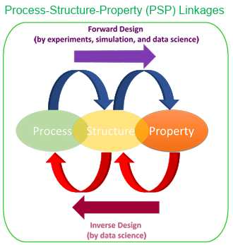
Figure 1.1 Schematic of materials design workflow by forward and inverse design using PSP linkages.
The use of microstructure images in ML modeling is challenging. The microstructure quantification has been reported as the central nucleus in the PSP linkages construction [37]. Microstructure quantification is important from two perspectives. First, it can increase the accuracy of the developed data-driven model. Second, an in-depth understanding of the microstructures can improve the comprehension of the effects of process variables and chemical composition on the properties of materials [37]. In recent years, deep learning (DL) methods have been successfully used in other fields, such as computer vision. Their limited applications in materials science have also proven them as reliable and promising methods [38]. The main advantages of DL methods are their simplicity, flexibility, and applicability for all types of microstructures. Furthermore, DL has been broadly applied in materials science to improve the targeted properties [34, 39 46].
One form of DL models that has been extensively used for feature extraction in various applications such as image, video, voice, and natural language processing is Convolutional Neural Networks (CNN) [47-50]. In materials science, CNN has been used for various image-related problems. Cang et al. used CNN to achieve a 1000-fold dimension reduction from the microstructure space [51]. DeCost et al. [52] applied CNN for microstructure segmentation. Xie and Grossman [53] used CNN to quantify the crystal graphs to predict the material properties. Their developed framework was able to predict eight different material properties such as formation energy, bandgap, and shear moduli with high accuracy. CNN has also been employed to index the electron backscatter diffraction patterns and determine the crystalline materials’ crystal orientation [54].
The stiffness in two-phase composites has been predicted successfully by the deep learning approach, including convolutional and fully-connected layers [55]. In a comparative study, the CNN and the materials knowledge systems (MKS), proposed in the Kalidindi group based on the idea of using the n-point correlation method for microstructures quantification [56-58], were used for microstructure quantification and then, the produced data were employed to predict the strain in the microstructural volume elements. The comparison showed that the extracted features by CNN could provide more accurate predictions [59]. Cecen et al. [20] proposed CNN to find the salient features of a collection of 5900 microstructures. The results showed that the obtained features from CNN could predict the properties more accurately than the 2-point correlation, while the computation cost was also significantly reduced. Comparing DL approaches, including CNN, with the MKS method, single-agent, and multi-agent methods shows that DL always performs more accurately [59-61]. Zhao et al. utilized the electronic charge density (ECD) as a generic unified 3D descriptor for elasticity prediction.
The results showed a better prediction power for bulk modulus than for shear modulus [62]. CNN has also been applied for finding universal 3D voxel descriptors to predict the target properties of the solid-state material [63]. The introduced descriptors outperformed the other descriptors in the prediction of Hartree energies for solid-state materials.
Training a deep CNN usually requires an extensive training dataset that is not always available in many applications. Therefore, a transfer learning method that uses a pretrained network can be applied for new applications. In transfer learning, all or a part of the pretrained networks such as VGG16, VGG19 [64], Xception [65], ResNet [66], and Inception [67], which were trained by the computer vision research community with lots of open source image datasets such as ImageNet, MS, CoCo, and Pascal, can be used for the desired application. In particular, in materials science which generally the image based data are not greatly abundant, transfer learning could be beneficial. DeCost et al. [68] adopted VGG16 to classify the microstructures based on their annealing conditions. Ling et al. [25] applied VGG16 to extract the feature from scanning electron microscope (SEM) images and classify them. Lubbers et al. [69] used the VGG 19 pretrained model to identify the physical meaningful descriptors in microstructures. Li et al. [70] proposed a framework based on VGG19 for microstructure reconstruction and structure-property predictions. The pretrained VGG19 network was also utilized to reconstruct the 3D microstructures from 2D microstructures by Bostanabad [71].
Review provided above shows that the majority of the ML-microstructure related works in the materials science community were primarily focused on using ML techniques for microstructure classification [72-74], recognition [75], microstructure reconstruction [70, 71], or as a feature-engineering-free framework to connect microstructure to the properties of the materials [55, 76, 77]. However, the process and chemistry prediction from a microstructure morphology image has received limited attention.
This is a critical knowledge gap to address specifically for the problems in them the ideal microstructure or morphology with the specific chemistry associated with the morphology domains are known, but the chemistry and processing which would lead to that ideal morphology is unknown. The problem becomes much more challenging for multicomponent alloys with complex processing steps. Recently, Kautz et al. [77] have used the CNN for microstructure classification and segmentation on Uranium alloyed with 10 wt% molybdenum (U-10Mo). They used the segmentation algorithm to calculate the area fraction of the lamellar transformation products of α-U + γ-UMo, and by feeding the total area fraction into the Johnson-Mehl-Avrami-Kolmogorov equation, they were able to predict the annealing parameters, i.e., time and temperature. However, Kautz et al.’s [77] work for aging time prediction did not consider the morphology and particle distribution, and also, no chemistry was involved in the model.
To address the knowledge gap, in this work, we develop a mixed-data deep neural network that is capable to predict the chemistry and processing history of a micrograph. The model alloy used in this work is Fe-Cr-Co permanent magnets.
Materials Microstructure Evolution Prediction
The processing-structure-property relationship of engineered materials is directly impacted by material microstructures, which are mesoscale structural elements that operate as an essential link between atomistic building components and macroscopic qualities. One of the pillars of contemporary materials research is the ability to manage the evolution of the material’s microstructure while it is being processed or used, including common phenomena like solidification, solid-state phase transitions, and grain growth.
Therefore, a key objective of computational materials design has been comprehending and forecasting of microstructure evolution. Simulations of microstructure evolution frequently rely on phase separation or coarse-grained models, such as partial differential equations (PDEs), which are used in the phase-field techniques [2, 78] because they can represent time and length scales that are far larger than those that can be captured by molecular dynamics. A wide range of significant evolutionary mesoscale processes, including grain development and coarsening, solidification, thin film deposition, dislocation dynamics, vesicle formation in biological membranes, and crack propagation, have all been fully described using the phase-field method [3-8].
However, there are some significant problems with this strategy as well. First off, PDE based microstructure simulations are still relatively expensive. The stability of numerical techniques that use explicit time integration for nonlinear PDEs sets stringent upper bounds on the smallest time-step size in the temporal dimension. Similarly, implicit time-integration techniques manage longer time steps by adding more inner iteration loops at each step. Furthermore, despite the fact that in theory controlling PDEs can be inferred from the underlying thermodynamic and kinetic considerations, actual PDE identification, parametrization, and validation take a significant amount of work.
The evolution principles may not be fully understood or may be too complex to be characterized by tractable PDEs for difficult or less well-studied materials. Currently, the efforts to reduce computational costs have mostly concentrated on utilizing high-performance computer architectures [79-82] and sophisticated numerical techniques [83, 84], or on merging machine learning algorithms with simulations based on microstructures [43, 85-91]. Leading studies, for instance, have developed surrogate models using a variety of techniques, such as Green’s function solution [85], Bayesian optimization [43, 86], a combination of dimensionality reduction and autoregressive Gaussian processes [88], convolutional autoencoder and decoder [92], or integrating a history-dependent machine-learning method with a statistically representative, low dimensional description of the microstructure evolution generated directly from phase-field simulations that can quickly predict the evolution of the microstructure from phase-field simulations [9].
The main problem, however, has been to strike a balance between accuracy and computing efficiency, even for these successful systems. For complex, multi-variable phase-field models, for example, precise answers cannot be guaranteed by the computationally effective Green’s function solution. In contrast, complex, coupled phase-field equations can be solved using Bayesian optimization techniques, however, at a higher computational cost (although the number of simulations required is kept to a minimum because the Bayesian optimization protocol determines the parameter settings for each subsequent simulation). The capacity of this class of models to predict future values outside of the training set is constrained by the fact that autoregressive models can only forecast microstructural evolution for the values for which they were trained. In other models based on dimensionality reduction methods like principle component analysis (PCA), a large amount of information is ignored, which will sacrifice accuracy. This study uses Predictive Recurrent Neural Network (PredRNN) [93] to forecast how the microstructure represented by 2D image sequences will change over time.
Dissertation Structure
The dissertation outline is as follows. In chapter two, we describe the methods used in this study, like PF, deep learning methods, train and test data generation, and error metrics.
In chapter three, we develop a mixed-data deep neural network capable of predicting a micrograph’s chemistry and processing history. The model alloy used in this work is Fe-Cr-Co permanent magnets. These alloys experience spinodal decomposition at temperatures around 853 – 963 K. We use the PF method to create the training and test dataset for the DL network. CNN will quantify the produced microstructures by the PF method; then the salient features will be used by another deep neural network to predict the temperature and chemical composition.
In chapter four, we explain a model based on a deep neural network to predict a complete set of processing parameters, including temperature, time, and chemistry from a micro structure micrograph. As a case study, we focused on the spinodal decomposition process, and to prove the model applicability for realistic alloys, we picked the Fe-Cr-Co permanent magnets as the model alloy. We used the PF method to create the training and test datasets for deep network training. A fused dataset including material microstructure as well as minimum and maximum iron concentration in the microstructure is used as the input data. We quantified the generated microstructures with the CNN and then combined the extracted salient features from the microstructures with iron composition to predict the processing history, i.e., annealing time and temperature, and chemical compositions of the micrograph.
In chapter five, we describe the microstructure evolution prediction by PredRNN. In this study, spinodal decomposition is used as a case study. Spinodal decomposition occurs in two separate phases: a quick composition modulation growth phase, followed by a slower coarsening phase, during which the Gibbs-Thomson effect causes a progressive rise in the length scale of the phase-separation pattern. We demonstrate that PredRNN can precisely capture all the required features from earlier microstructures to predict long-term microstructures. This result is particularly important because it can predict morphology evolution in both phases.
Finally, the key findings in this thesis are summarized and possible opportunities for future works are discussed.
This dissertation leads to the following peer-reviewed and conference papers;
1. Amir Abbas Kazemzadeh Farizhandi, Mahmood Mamivand, Processing time, temperature, and initial chemical composition prediction from materials microstructure by deep network for multiple inputs and fused data, Materials &
Design, Volume 219, 2022, 110799, ISSN 0264-1275,
https://doi.org/10.1016/j.matdes.2022.110799.
2. Amir Abbas Kazemzadeh Farizhandi, Omar Betancourt, Mahmood Mamivand. Deep learning approach for chemistry and processing history prediction from materials microstructure. Sci Rep 12, 4552 (2022).
https://doi.org/10.1038/s41598-022-08484-7.
3. Amir Abbas Kazemzadeh Farizhandi, Mahmood Mamivand, Spatiotemporal Prediction of Microstructure Evolution with Predictive Recurrent Neural Network, Submitted to Materials & Design.
4. Amir Abbas Kazemzadeh Farizhandi, Mahmood Mamivand, Chemistry and Processing History Prediction from Materials Microstructure by Deep Learning, 2022 TMS Annual Meeting & Exhibition, Symposium: Algorithm Development in Materials Science and Engineering.
5. Amir Abbas Kazemzadeh Farizhandi, Mahmood Mamivand, Spatiotemporal Prediction of Microstructure by Deep Learning, 2022 TMS Annual Meeting & Exhibition, Symposium: AI/Data Informatics: Computational Model Development, Validation, and Uncertainty Quantification.
6. Smith, Leo, Mahmood Mamivand, Amir Abbas Kazemzadeh Farizhandi, and Carl Agren. “Prediction of Onsager and Gradient Energy Coefficients from Microstructure Images with Machine Learning.” Idaho Conference on Undergraduate Research (2022).
7. Keynote Speaker: Mahmood Mamivand, Amir Abbas Kazemzadeh, “Microstructural mediated materials design with deep learning”, International Conference on Plasticity, Damage, and Fracture, Jan 2023
8. Invited Talk: Mahmood Mamivand, Amir Abbas Kazemzadeh, “Chemistry and Processing History Prediction from Microstructure Morphologies”, TMS March 2023
CHAPTER TWO: METHOD
In this chapter, we describe the models and algorithms that we have used in this dissertation. First, we briefly describe the Phase Field (PF) model for spinodal decomposition simulation and the dataset generation process. Then, we provide the details of the proposed fused-data deep neural network for process history and chemistry prediction from materials microstructure morphologies. Finally, we explain the LSTM model that has been used to predict the evolution of material microstructures along with an overview of methods to quantify the similarity between microstructure morphologies.
Phase Field Method
With the enormous increase in computational power and advances in numerical methods, the PF approach has become a powerful tool for the quantitative modeling of microstructures’ temporal and spatial evolution. Some applications of this method include modeling materials undergoing martensitic transformation [94], crack propagation [95], grain growth [96], and materials microstructure prediction for optimization of their properties [97].
The PF method eliminates the need for the system to track each moving boundary by having the interfaces to be of finite width where they gradually transform from one composition or phase to another [2]. This essentially causes the system to be modeled as a diffusivity problem, which can be solved by using the continuum nonlinear PDEs. There are two main PF PDEs for representing the evolution of various PF variables. One being the Allen-Cahn equation [98] for solving non-conserved order parameters (e.g., phase regions and grains), and the other one being the Cahn-Hilliard equation [99] for solving conserved order parameters (e.g., concentrations).
Since the diffusion of constituent elements controls the process of phase separation, we only need to track the conserved variables, i.e., Fe, Cr, and Co concentration, during isothermal spinodal phase decomposition. Thus, our model will be governed by Cahn Hilliard equations. The PF model in this work is primarily adopted from [100]. For the spinodal decomposition of the Fe-Cr-Co ternary system, the Cahn-Hilliard equations are,
𝜕𝑐𝑐r by at=∇⋅𝑀 c r.c r∇⋅ 𝛿𝐹𝑡o𝑡by 𝛿𝑐𝑐r+∇⋅𝑀cr,co∇𝛿𝐹𝑡o𝑡by 𝛿𝑐𝑐o, (1)
𝜕𝑐𝑐o by at=∇⋅𝑀 c o.c r∇⋅ 𝛿𝐹𝑡o𝑡by 𝛿𝑐𝑐r+∇⋅𝑀co,co∇𝛿𝐹𝑡o𝑡by 𝛿𝑐𝑐o. (2)
The microstructure evolution is primarily driven by the minimization of the total free energy Ftot of the system. The free energy functional, using N conserved variables ci at the location 𝑟𝑟⃗ is described by:
Ftot = ∫𝑟⃗ [ 𝑓𝑙oc (𝑐1,…,𝑐𝑁,𝑇)+𝑓𝑔𝑟(𝑐1,…,𝑐𝑁,)]𝑑𝑟⃗ 𝐸𝑒𝑙. (3)
𝑓𝑔r=kby2∑Ni |∇𝑐|2, (4)
where κi is the gradient energy coefficient. In this case, κ is considered a constant value. floc is the local Gibbs free energy density as a function of all concentrations, ci, and temperature, T. For this work, we will model the body-centered cubic phase of Fe-Cr-Co, where the Gibbs free energy of the system is described as [100],
𝑓𝑙o𝑐=𝑓0𝐹e 𝐶𝐹𝑒+𝑓0cr ccr+𝑓0co cco+𝑅𝑇(𝐶𝐹𝑒inc 𝐹e+ccr inc cr +cco inc co)+𝑓𝑒+𝑓mg, (5)
where fi 0 is the Gibbs free energy of the pure element i and fE is the excess free energy defined by
𝑓𝐸=𝐿𝐹𝑒,cr 𝐶𝐹𝑒 ccr +𝐿𝐹e,co𝐶𝐹ecco +𝐿𝐶r,cocr cco, (6)
where LFe,Cr, LFe,Co, and LCr,Co are interaction parameters. fmg is the magnetic energy contribution and can be expressed as
𝑓𝑚𝑔+𝑅𝑇In(β+1)𝑓(𝜏), (7)
where β is the atomic magnetic moment, f(τ) is a function of τ ≡ T/TC. TC is the Curie temperature. Eel in Eq. (3) is the elastic strain energy added to the system and is expressed as
𝐸𝑒𝑙+1by2∫ 𝑟⃗𝐶𝑖 jkl 𝜀 el kl (𝑟⃗,t)d𝑟⃗, (8)
𝜀el ij (𝑟⃗, 𝑡)=𝜀cij (𝑟⃗,t)-𝜀0j(𝑟⃗, 𝑡), (9)
𝜀0ij(𝑟⃗, 𝑡)=[𝜀cr(ccr(𝑟⃗, 𝑡)-c0cr)=𝜀co(cco(𝑟⃗, 𝑡)-c0co)]𝛿𝑖j, (10)
where 𝜀cr and 𝜀co are lattice mismatches between Cr with Fe and Co with Fe,
respectively. 𝐶0𝑐andC0c0 are the initial concentrations of Cr and Co, respectively and 𝛿𝑖j is the Kronecker delta. The constrained strain, 𝜀𝑖j(𝑟⃗, 𝑡),is solved using the finite element method. 𝑀𝑖j in Eq. (2) are Onsager coefficients and are scalar mobilities from the coupled system involving the concentrations. They can be determined by [100],
𝑀𝐶r,𝐶r = [𝑐𝐹𝑒 ccr𝑒 𝑀𝐹+ (1 −𝐶cr)2𝑀cr+ccr cco 𝑀co] 𝐶𝐶rby rt, (11)
𝑀co,co=[CfeCco Mfe+ccr cco Mcr+(1-Cco)2 Mco]Ccobyrt, (12)
MCr Co = MCo.cr =𝑀Co ,cr=[Cfe,Mfe- (1− Cr)MCr-(1− Cco)MCo]CCr Cco by rt
(13)
The mobility Mi of each element i is determined by
Mi=D0i exp (-Qi by KBT), (14)
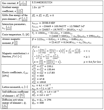
where 𝐷0i is the self-diffusion coefficient and 𝑄𝑄𝑖𝑖 is the diffusion activation energy. We parametrized the model with the calculation of phase diagram (CALPHAD) data [100]. To solve the non-linear CH partial differential equations (PDEs), we used the Multi-physics Object-Oriented Simulation Environment (MOOSE). MOOSE is an open source finite element package developed at Idaho National Laboratory and efficient for parallel computation on supercomputers [101]. The coupled CH equations were solved with the help of MOOSE’s prebuilt series of weak form residuals of CH PDEs with the input parameters given in Table 2.1.
Table 2.1 Phase-field model input parameters [100, 102, 103]
Dataset Generation
Dataset Generation for Steady State Case Study
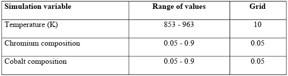
Since the compositions are subject to the constraint that they must sum to one, the dataset was produced based on the mixture design as a design of experiments method [104]. The Simplex-Lattice [105] designs were adopted to provide the data for simulation. The simulation variables and their range of values are given in Table 2.2. The simulations were run on Boise State University R2 cluster computers [106] using the MOOSE framework [101].
Table 2.2 Simulation variables and their range of values for database generation of steady state case study.
After running the simulations, the micro structures were collected from the results showing the phase separation. The extracted micro structures for Fe, i.e., the morphology of Fe distribution, from the PF simulations, along with the minimum and maximum compositions of Fe in each microstructure, are utilized as the inputs to predict spinodal temperature, Cr, and Co compositions as processing history parameters. Indeed, the input data is a mixed dataset combined of microstructures, as image data, and Fe composition, as numerical or continuous data. Since these values constitute different data types, the machine learning model must be able to ingest the mixed data. In general, handling the mixed data is challenging because each data type may require separate preprocessing steps, including scaling, normalization, and feature engineering [107].
Dataset Generation for Unsteady State Case Study
To develop proper training and test datasets, we need to span the possible ranges of input variables, i.e., time, temperature, and chemical compositions. For the temperature, we are bonded to the range of 850 – 970 K, as spinodal decomposition in Fe-Cr-Co happens in this window. For chemistry, we explore the range of 0.05-0.9 at. % for both Cr and Co.
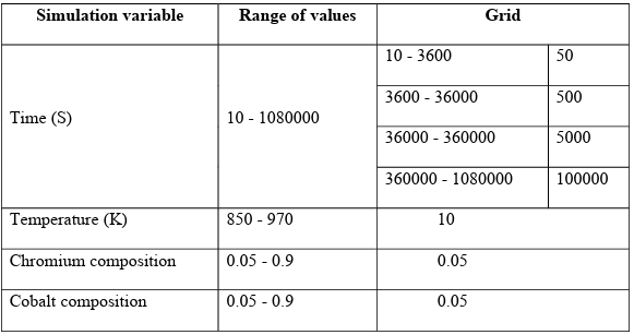
Since the chemistry is subjected to the conservation of mass constrain, i.e., cFe+cCr+cCo = 1, we used the Simplex-Lattice [105] as a mixture design method to generate the chemistry space to explore. Finally, we bounded the dataset to 300 hours for the time, as our study showed most microstructures would reach equilibrium to some extent by this time. Unlike temperature and chemistry, we did not grid the time domain linearly because the microstructure is very sensitive to aging time in the early stages of annealing, but this sensitivity drops dramatically as time passes. Therefore, we picked a fine grid at the beginning, 50 s, and increased it exponentially, to 100000 s, with time.
The variables and their ranges are given in Table 2.3. To cover all the range of input variables, the dataset was generated based on the design of the experiment (DOE). We generated the microstructures by solving the CH PDEs using the MOOSE framework [101]. The simulations were run on different clusters including Boise State University R2 cluster computers [106], Boise State University BORAH [108], and the Extreme Science and Engineering Discovery Environment (XSEDE) (Jetstream2 cluster), which is supported by National Science Foundation (NSF) [109] using the MOOSE framework [101]. We note that because of the deterministic nature of the PF technique, i.e., not being stochastic, and the physics of the spinodal decomposition, we only need to run each condition once.
Table 2.3 Simulation variables and their range of values for database generation of unsteady state case study.
After simulations, we collected the morphology of Fe distribution, which represents the Fe-rich and Fe-depleted, i.e., Cr-rich, regions, as image data. In addition, we used the minimum and maximum compositions of Fe in each microstructure as numeric data. The deep network uses images and numeric data as input to predict the time, temperature, and chemical compositions. Therefore, different types of deep networks like convolutional and fully-connected layers are required to process the input data. We note that the accuracy of the model will increase for real materials if some experimental data is added to the training dataset. However, even having the experimental dataset to be just a few percent of the whole dataset, requires hundreds of tailored transmission electron microscopy (TEM) images. Generating such a big experimental dataset is time consuming and costly. Therefore, in this work, we limit the model to synthetic data. 23 However, as we will show in the validation part, the model predicts the history of an experimental TEM image pretty well, because we are using a CALPHAD-informed phase field model to generate the training and test dataset, and CALPHAD is inherently informed by some experimental data.
Dataset Generation for Microstructure Evolution Case Study
The produced microstructures in the unsteady state case study are also used as training, validation, and test data in this study. The Fe-based composition microstructure morphologies sequences are utilized to construct the dataset. The length of each sequence is 20 microstructures; the first 10 microstructures until 30 hr of the process are used to predict the future 10 microstructures until 300 hr.
Deep Learning Methodology
Deep learning (DL), as an artificial intelligence (AI) tool, is usually used for image and natural language processing as well as object and speech recognition based on human brain mimicking [49, 110]. Indeed, DL is a deep neural network that can be applied for supervised, e.g., classification and regression tasks, and unsupervised, e.g., clustering, learning. In this work, since we have two different data types as input, two various networks are needed for data processing. The numerical data is fed into fully-connected layers while image features are extracted through the convolutional layers. For images involving a large number of pixel values, it is often not feasible to directly utilize all the pixel values for fully-connected layers because it can cause overfitting, increased complexity, and difficulty in model convergence. Hence, convolutional layers are applied to reduce the dimensionality of the image data by finding the image features [73, 111].
Fully-Connected Layers
Fully-connected layers are hidden layers consist of hidden neurons and activation function [112]. The number of hidden neurons is usually selected based on trial and error.
The neural networks can predict complex nonlinear behaviors of systems through activation functions. Any nonlinear function that is differentiable can be used as an activation function. However, there are some activation functions such as rectified linear (ReLU), leaky rectified linear, hyperbolic tangent (Tanh), sigmoid, Swish, and softmax that have been successfully used in different applications in neural networks [113]. In particular, ReLU (f(x) = max (0, x)) and Swish (f(x) = x sigmoid(x)) activation functions have been recommended for hidden layers in deep neural networks [114].
Convolutional Neural Networks (CNN)
A convolutional neural network (CNN) is a deep network that is applied for image processing and computer vision tasks. For the first time, LeCun et al. proposed using CNN for image recognition [115]. CNN, like other deep neural networks, consists of input, output, and hidden layers. But the main difference lies in the use of hidden layers consisting of convolutional, pooling, and fully-connected layers that follow each other. Several convolutional and pooling layers can be designed in the CNN architectures. Convolutional layers can extract the salient features of images without losing the information. At the same time, the dimensionality of the generated data gets reduced and then fed as input to the fully-connected layer. Two significant advantages of CNN are parameter sharing and sparsity of the connections. A schematic diagram for CNN is given in Figure 2.1.
The convolutional layer consists of filters that pass over the image and scanning the pixel values to make a feature map. The produced map proceeds through the activation function to add nonlinearity property. The pooling layer involves a pooling operation, e.g., maximum or average, which acts as a filter on the feature map. The pooling layer reduces the size of the feature map by pooling operation. Different combinations of convolutional and pooling layers are usually used in various CNN architectures. Finally, the fully-connected layers are added to train on image extracted features for a particular task such as classification or regression.
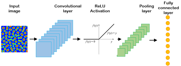
Figure 2.1
Schematic of a typical convolutional neural network.
Similar to other neural networks, a cost function is used to train a CNN and update the weights and biases by back propagation. There are many hyperparameters such as the number of filters, size of filters, regularization values, dropout values, optimizer parameters, initial weights, and biases that must be initialized before training. Training a
CNN usually needs an extensive training dataset that is not always available for all applications. In this situation, transfer learning can be helpful in developing a CNN. In transfer learning, all or part of a pretrained network like VGG16, VGG19 [64], Xception [65], ResNet [66], and Inception [67], which were trained by computer vision research community with lots of open source image datasets such as ImageNet, MS, CoCo, and Pascal, can be used for the desired application. The state-of-the-art pretrained network is EfficientNet which was proposed by Tan and Le [116].
This method is based on the idea that scaling up the CNN can increase its accuracy [117]. Since there was no complete understanding of the effect of network enlargement on the accuracy, Tan and Le proposed a systematic approach for scaling up the CNNs. There are different ways to scale up the CNNs by their depth [117], width [118], and resolution [119]. Tan and Le proposed to scale up all the depth, width, and resolution factors for the CNN with fixed scaling coefficients. [116]. The results demonstrated that their proposed network, EfficientNet-B7, had better accuracy than the best-existing networks while using 8.4 times fewer parameters and performing 6.1 times faster. In addition, they provided other EfficientNet-B0 to -B6, which can overcome the models with the corresponding scale such as ResNet-152 [117] and AmoebaNet-C [120] in terms of accuracy with much fewer parameters. Due to the outstanding performance of EfficientNet, although it is trained based on the ImageNet dataset which is completely different from materials micro structures, it seems the EfficientNets convolutional layers have the potential to extract the features of images from other sources like materials micro structures.
Proposed Model for Steady State Case Study
The training and test datasets are produced using the PF method. In this work, two different algorithms, including CNN and transfer learning, were proposed to extract the salient features of the microstructure morphologies. We applied a proposed CNN (Figure 2.2) or part of pretrained EfficienctNet B-6 and B-7 convolutional layers (Figure 2.3) to find the features of the microstructures. The architecture of the proposed CNN was found by testing different combinations of convolutional layers and their parameters based on the best accuracy. In the transfer learning part, different layers of the pretrained convolutional layers were tested to find the best convolutional layers for feature extraction.
On the other hand, the minimum and maximum Fe composition in the microstructure, as numerical data, is fed into the fully-connected layers. The extracted features from micro structures and the output of the fully-connected layers are combined to feed other fully-connected layers to predict the processing temperature and initial Cr and Co compositions. Different hyper parameters such as network architecture, cost function, and optimizer are tested to find the model with the highest accuracy. The model specifications, compilations (here loss function, optimizer, and metrics), and cross validation parameters are listed in Table 2.4.
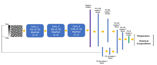
Figure 2.2
The flowchart of the developed model for chemistry and processing
history prediction from microstructure images (FC: fully-connected layer)
Table 2.4 Parameters selected for model specification, compilation, and cross validation.

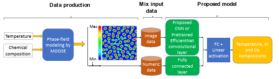
Figure 2.3 The flowchart of the developed model for chemistry and processing
history prediction from microstructure images (FC: fully-connected layer)
Proposed Model for Unsteady State Case Study
In this study, different in-house CNNs or different layers of pretrained convolutional layers of Efficient Net have been adopted to extract microstructure features. The proposed deep network in the framework includes different in-house CNNs or pretrained convolutional layers from EfficientNet-B7 (transfer learning) for micro structure feature extraction and fully-connected layers for processing of the extracted features and numeric data (Iron minimum and maximum composition in the micrographs). CNNs with different convolutional layers are applied for microstructure feature extraction in the in house CNNs. In transfer learning, different layers of pretrained convolutional networks are tested to find the optimum number of layers based on the overall accuracy.
The architecture of the proposed network is found by testing different combinations of convolutional, fully-connected layers and their parameters based on the best accuracy. A schematic flowchart of the proposed framework is given in Figure 2.4. The extracted features of microstructures are passed through fully-connected layers to get combined with the output of the fully-connected layers that proceed the numeric data. The network is trained by the end-to-end method to find the optimum hyperparameters. The model parameters and specifications are the same as in Table 2.4, and only the output dimension will be 4.
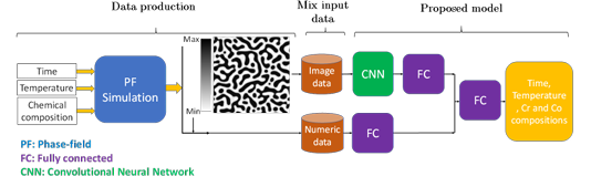
Figure 2.4
The flowchart of the developed model for chemistry, time, and
temperature prediction from microstructure images (FC: fully-connected layer)
Proposed Model for Micro structure Evolution Prediction
Prediction of microstructure evolution is a spatiotemporal problem. Different network architectures, which can generally be grouped into three categories: feed-forward models based on CNNs, recurrent models, and others such as the combinations of convolution and recurrent networks, as well as the Transformer-based and flow-based methods, are used to encode different inductive biases into neural networks for spatiotemporal predictive learning [121]. The inductive bias of group invariance over space has been brought to spatiotemporal predictive learning through the use of convolutional layers. For next frame prediction in Atari games, Oh et al. [122] defined an action-conditioned autoencoder with convolutions. The Cross Convolutional Network, developed by Xue et al. [123], is a probabilistic model that stores motion data as convolutional kernels and learns to predict a likely set of future frames by understanding their conditional distribution. In order to complete the crowd flow prediction challenge, Zhang et al. [124] suggested using CNNs with residual connections. It specifically takes into account the proximity, duration, trend, and external elements that affect how population flows move. Additionally, the convolutional architectures are employed in tandem with the generative adversarial networks (GANs) [125], which successfully lowered the learning process’ uncertainty and enhanced the sharpness of the generated frames. Most feed-forward models demonstrate greater parallel computing efficiency on large-scale GPUs compared to recurrent models [126-128].
However, these models generally fail to represent long term reliance across distant frames since they learn complex state transition functions as combinations of simpler ones by stacking convolutional layers.
Some helpful insights into how to forecast upcoming visual sequences based on historical observations are provided by recent developments in RNNs. In order to forecast future frames in a discrete space of patch clusters, Ranzato et al. [129] built an RNN architecture that was influenced by language modeling. As a remedy for video prediction, Srivastava et al. [130] used a sequence-to-sequence LSTM model from neural machine translation [131]. Later, other approaches to describe temporal uncertainty or the multimodal distribution of future frames conditioned on historical observations have been presented, by integrating variational inference with 2D recurrence [132-135].
By arranging 2D recurrent states in hierarchical designs, certain additional techniques successfully increased the forecast time horizon [136]. The factorization of video information and motion is another area of research, typically using sequence-level characteristics and temporally updated RNN states [137]. The use of optical flows, new adversarial training schemes, relational reasoning between object-centric content and pose vectors, differentiable clustering techniques, amortized inference enlightened by unsupervised image decomposition, and new types of recurrent units constrained by partial differential equations are typical approaches [138-143]. The aforementioned techniques work well for breaking down dynamic visual scenes or understanding the conditional distribution of upcoming frames. To describe the spatiotemporal dynamics in low-dimensional space, they primarily use 2D recurrent networks, which inadvertently results in the loss of visual information in actual circumstances.
Shi et al. [144] created the Convolutional LSTM (ConvLSTM), which substitutes convolutions for matrix multiplication in the recurrent transitions of the original LSTM to combine the benefits of convolutional and recurrent architectures. An action-conditioned ConvLSTM network was created by Finn et al. [145] for visual planning and control.
Shi et al. [146] coupled convolutions with GRUs and used non-local neural connections to expand the receptive fields of state-to-state transitions. Wang et al. [147] introduced a higher-order convolutional RNN that uses 3D convolutions and temporal self-attention to describe the dynamics and includes a time dimension in each hidden state. Su et al. [148] increased the low-rank tensor factorization-based higher-order ConvLSTMs’ computational effectiveness. Convolutional recurrence provides a platform for further research by simultaneously modeling visual appearances and temporal dynamics [149 154]. The spatiotemporal memory flow, a novel convolutional recurrent unit with a pair of decoupled memory cells, and a new training method for sequence-to-sequence predictive learning are all used to enhance the existing architectures for action-free and action-conditioned video prediction in Predictive Recurrent Neural Network (PredRNN) [93].
A network component known as a memory cell is crucial in helping stacked LSTMs solve the vanishing gradient issue seen by RNNs. It can latch the gradients of hidden states inside each LSTM unit during training, preserving important information about the underlying temporal dynamics, according to strong theoretical and empirical evidence.
However, the spatiotemporal predictive learning task necessitates a distinct focus on the learned representations in many areas from other tasks of sequential data; therefore, the state transition pathway of LSTM memory cells may not be optimum. First, rather than capturing spatial deformations of visual appearance, most predictive networks for language or speech modeling concentrate on capturing the long-term, non-Markovian features of sequential data [155, 156]. However, both space-time data structures are essential and must be carefully considered in order to forecast future frames.
Second, low-level features are less significant to outputs in other supervised tasks using video data, such as action recognition, where high-level semantical features may be informative enough. The stacked LSTMs don’t have to maintain fine-grained representations from the bottom up because there are no complex structures of supervision signals. Although the current inner-layer memory transition-based recurrent architecture can be sufficient to capture temporal variations at each level of the network, it might not be the best option for predictive learning, where low-level specifics and high-level semantics of spatiotemporal data are both significant to generating future frames. Wang et al.
[93] proposed a new memory prediction framework called PredRNN, which extends the inner layer transition function of memory states in LSTMs to spatiotemporal memory flow.
This framework aims to jointly model the spatial correlations and temporal dynamics at different levels of RNNs. All PredRNN nodes are traversed by the spatiotemporal memory flow in a zigzag pattern of bi-directional hierarchies: A newly created memory cell is used to deliver low-level information from the input to the output at each time step, and at the top layer, the spatiotemporal memory flow transports the high-level memory state to the bottom layer at the following timestep. The Spatiotemporal LSTM (ST LSTM), in which the proposed spatiotemporal memory flow interacts with the original, unidirectional memory state of LSTMs, was therefore established as the fundamental building element of PredRNN.
It seems that they would require a unified memory mechanism to handle both short-term deformations of spatial details and long-term dynamics if they anticipated a vivid imagination of numerous future images: On the one hand, the network may learn complex transition functions within brief neighborhoods of subsequent frames thanks to the new spatiotemporal memory cell architecture, which also increases the depth of nonlinear neurons across time-adjacent RNN states. Thus, it considerably raises ST-modeling LSTM’s capacity for short-term dynamics. To achieve both long-term coherence of concealed states and their fast reaction to short-term dynamics, ST-LSTM, on the other hand, still uses the temporal memory cell of LSTMs and closely combines it with the suggested spatiotemporal memory cell. Schematics of the PredRNN architecture and the ST-LSTM unit with twisted memory states are given in Figure 2.5.
On five datasets—the Moving MNIST dataset, the KTH action dataset, a radar echo dataset for precipitation forecasting, the Traffic4Cast dataset of high-resolution traffic flows, and the action-conditioned BAIR dataset with robot-object interactions—the proposed methodology demonstrated state-of-the-art performance. The original paper [93] contains information about the investigation in detail. This dissertation adopts the PredRNN to predict the microstructure evolution in a split second.
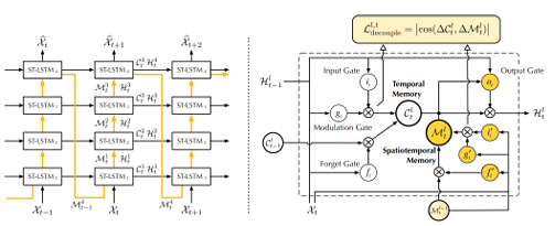
Figure 2.5 Left: the main architecture of PredRNN, in which the orange arrows denote the state transition paths of Ml t, namely the spatiotemporal memory flow. Right: the ST LSTM unit with twisted memory states serves as the building block of the proposed PredRNN, where the orange circles denote the unique structures compared with ConvLSTM (the figure was adopted from the original study [157]).
Measure the Similarity Between Images
Perhaps the most fundamental process underpinning all of computing is the capability to compare data elements. It is not particularly challenging in many fields of computer science; for example, binary patterns may be compared using the Hamming distance, text files can be compared using the edit distance, vectors can be compared using the Euclidean distance, etc. Even the seemingly straightforward operation of comparing visual patterns is still an open problem, which makes computer vision a particularly difficult field to study. Visual patterns are not just exceedingly high-dimensional and strongly correlated, but the idea of visual similarity itself is frequently arbitrary and intended to emulate human visual perception [158]. In order to compare the various outcomes of the experiments when working on computer vision tasks, we must select a method for measuring the similarity between two images. Objective quality or distortion assessment techniques can be divided into two main categories. The first category includes metrics that may be expressed quantitatively, such as the frequently used mean square error (MSE), peak signal to noise ratio (PSNR), root mean square error (RMSE), mean absolute error (MAE), and signal-to-noise ratio (SNR). In an effort to include measurements of perceptual quality, the second class of measurement techniques takes into account the properties of the human visual system (HVS) [159].
The mean-square error estimator is the most common. The average squared difference between the anticipated values (estimated values) and the actual value is measured by MSE (ground truth). Therefore, we just square the differences between each pixel. However, this only works well if we want to create a picture with the best pixel colors consistent with the real-world image. We occasionally like to focus on the picture’s structure or relief [158].
The second conventional estimator is PSNR (Peak Signal to Noise Ratio). All pixel representation values must be converted to bit form to utilize this estimator. The values of the pixel channels must range from 0 to 255 if we are using 8-bit pixels. By the way, the RGB color model, sometimes known as red, green, and blue, suits the PSNR the best.
The PSNR metric displays the relationship between a signal’s maximum achievable power and the power of corrupting noise that compromises the accuracy of its representation [159].
However, PSNR, a variant of MSE, continues to focus on the pixel-by-pixel comparison. Another technique for image similarity quantification is the structural similarity approach (SSIM). SSIM and the effectiveness and perception of the human visual system are connected (HVS color model). The SSIM represents picture distortion as a combination of three elements, namely loss of correlation, luminance distortion, and contrast distortion, as opposed to utilizing conventional error summation techniques [159].
Convolutional neural networks’ hidden variables have recently been demonstrated to be an effective measure of perceptual similarity that accurately predicts human perception of relative picture similarity. The perceptual similarity between two images is assessed using the Learned Perceptual Image Patch Similarity (LPIPS). In essence, LPIPS determines how comparable two picture patches’ activations are for a given network. This measurement has been demonstrated to reflect human perception closely. Image patches with a low LPIPS score are perceptually similar [158].
In material science, there are other methods for microstructure assessment, including two-point correlation function, chord length distribution, etc. In addition to index values such as MSE, PSNR, SSIM, and LPIPS, two-point correlation function [160] and chord length [161] are used for distribution comparison between two images in this dissertation. In two-point correlation, the local state and local state space can be used to digitize the microstructure images [162]. Local space (h) is the attributes that are needed to completely identify all relevant material properties for the selected length scale and can be defined as follows:
ℎ =(𝜌,𝑐𝑖) (15)
Where ρ is a phase identifier (α, β, γ, …) and 𝑐𝑐𝑖𝑖 represents chemical composition. The complete set of all theoretically possible local states in a selected material system is the local state space (H) [163].
𝐻 ={(𝜌,𝑐𝑖)||𝜌 𝜀{𝛼,𝛽,𝛾,…},𝑐𝑖 𝜀𝐶𝑓i} (16)
Representation of the microstructure as a function h(x, t) specifies the local state present at every spatial position x and time t. In practice, all microstructure characterization techniques probe the local state in the materials over a finite volume and a finite time interval. It is impractical to implement this function in practice due to the resolution limits and uncertainty inherent to the characterization techniques used. In addition, the local state can only be characterized as an average measure over a finite probe volume and finite time step. The problem raises is the fact that the local state in any particular pixel or voxel at any particular time step may not be unique [164]. To solve the mentioned issues, microstructure function m(h, x) is defined as the probability density associated with finding local state h at the spatial location x at time t. It captures the probability of finding one of the local states that lie within a small interval dℎ centered around ℎ at a selected x. m(ℎ, x) dℎ dx would represent the probability and m(ℎ, x) the corresponding probability density [165]. The desired information for the evaluation of m(h, x) is usually discrete values.
The microstructure image on a square lattice can be represented by pixel in two dimensional (2D) images and voxel in three-dimensional (3D) images. In this case, the microstructure images are expressed by arrays that each element of the array has a value based on that pixel or voxel brightness. Then, enough sampling grid is needed to capture rich attributes from the material internal structure. The different phases in the material microstructure can be represented by special values. For example, Figure 2.6a shows a real two-phase microstructure that can be depicted by a binary image (black and white).
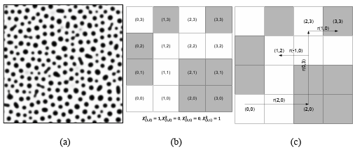
Figure 2.6 (a) A real two-phase micro structure, (b) and (c) a simple checkerboard microstructure for presenting X_uv and two-point correlation (white color is phase 1 and black color is phase 2)
If X indicates the micro structure on a square lattice, it can be displayed mathematically as follows:
𝑋𝑢v = {1, 0 ,𝑖𝑓u v ∈ phase 1 otherwise (17)
uv is the pixel index and represents the pixel location in the microstructure image. In the two-point correlation function, as a simple n-point correlation method, the correlation between two random points in the microstructure that can be specified by vector r are evaluated as follows:
𝑓r np,uv =〈Xnuv,Xpuv+ 〉 (18)
Where 〈.〉 is the expectation operator. A simple example for 𝑋𝑋𝑢𝑢𝑢𝑢 and two-point correlation has been presented in Figures 1b and 1c. Since we are dealing with discrete values, the expectation can be defined as:
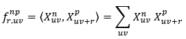
(19)
𝑓r𝑛𝑝 uv is the conditional probability of finding local state n at bin uv given finding local state p at bin uv+r. This definition can be extended for three, four, or n-point correlation function. If there is a periodic micro structure, 𝑓rnp,uv is independent from uv. For a two-phase material, there are 𝑓r11, 𝑓r12, 𝑓r21, and 𝑓r22.
𝑓r𝑛p=[fr11,fr12,fr21,fr22] (20)
The lineal-path function is an additional statistical function that can help for microstructure characterization. The lineal-path function quantifies the clusteredness of the straight lines in the microstructure. In fact, form probabilistic point of view, the probability that a line drawn on the microstructure will be completely in one phase is calculated [166, 167]. It can be calculated by different methods like chords distribution [166] or Monte Carlo simulation [168]. The lineal-path function in a microstructure is linearly independent unlike two-point correlation which is more effective for phases recognition. The second derivative of lineal-path function is chord-length distribution (CLD) which is also used for microstructure quantification [169]. The lineal-path function cannot show the connectivity of the phases accurately because just linear connections are considered in this method. In addition, these linear connections are measured in the certain directions. Some studies tried to apply different methods to evaluate it in the multiple directions [170-172]. Despite these weaknesses, the lineal-path function has been applied for micro structure characterization in different studies [166, 173]. The CLD function which can be derived from lineal-path function was used by Popova et al. [174] to quantify the material structure in additive manufacturing. Some researchers have reported that the lineal-path function and the two-point cluster correlation function is useful for finding clusters in the microstructures [166, 173, 175].
CHAPTER THREE: DEEP LEARNING APPROACH FOR CHEMISTRY AND PROCESSING HISTORY PREDICTION FROM MATERIALS MICROSTRUCTURE
In this chapter, we develop a deep neural network to predict chemistry and processing history prediction from materials microstructure. All the microstructures in this chapter belong to a heat treatment time of 100 hr. The result provided in this chapter is published as a research paper [176] in the Scientific Report Journal (Volume 12, 4552 (2022), https://doi.org/10.1038/s41598-022 08484-7).
Phase-Field Modeling and Dataset Generation
Different microstructures are produced by PF modeling for different chemical compositions and temperatures. The chemical compositions and temperature were designed based on the design of experiment method. Since the chemical compositions are subject to the constraint that they must sum to one, the Simplex-Lattice design as a standard mixture design was adopted to produce the samples. In this regard, the compositions start from 0.05 and increase to 0.90 at 0.05 intervals, and the temperature rises from 853 K to 963 K at 10 K increment, see Table 2.2. Therefore, 2053 different samples were simulated by the PF method, and the microstructures were constructed for different chemical compositions and temperatures. All the proposed operating conditions were simulated for the 100 hr spinodal decomposition process. Figure 3.1 depicts three sample results of the PF simulation. The MOOSE-generated data can be presented in different color formats. In most transmission electron microscopy (TEM) images in literature, the Fe-rich and Cr-rich phases have been shown by bright and dark contrasts, respectively. We followed the same coloring for the extracted microstructures from the MOOSE. The Chigger python library in MOOSE has been used for micro structures extraction.
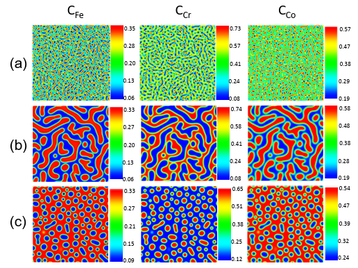
Figure 3.1
Fe-Cr-Co alloys microstructure generated by the phase-field method
for: a) Fe-20%, Cr-40%, Co-40% at 873K, b) Fe-20%, Cr-40%, Co-40% at 963K, c)
Fe-25%, Cr-30%, Co-45% at 933K. (Composition are in atomic percent).
Since decomposition does not occur in all the proposed operating conditions and chemistries, the microstructures showing the 0.05 difference in Fe composition between Cr-rich and Fe-rich phases were considered spinodally decomposed results. Hence, 454 samples in which decomposition has taken place are used to create the database. 80% of 454 samples were used for training and 20% for testing. The training was validated by 5 fold cross-validation. The Fe-based composition micro structure morphologies, as well as minimum and maximum of Fe compositions in the microstructure along with corresponding chemical compositions and temperatures, form the dataset. A sample workflow on the dataset construction is given in Figure 3.2.
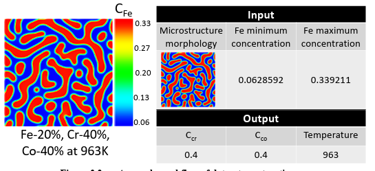
Figure 3.2
A sample workflow of dataset construction.
Convolutional Layers for Feature Extraction
The overreaching goal of the convolutional layers is feature extraction from the images. First, we train a proposed CNN, which includes three convolutional layers, batch normalization, max pooling, and ReLU activation function. Filters in each convolutional layer encode the salient features of images. Once the input images are fed into the network, the filters in the convolutional layers are activated to produce the response maps as an output of the filters. Some response maps of each convolutional layer in the proposed CNN are given in Figure 3.3.
Then, as a comparison, the EfficientNet-B6 and EfficientNet-B7 convolutional layers were also applied to extract the salient features of produced microstructure by the PF method. The EfficientNet-B6 and EfficientNet-B7 have 43 and 66 million parameters which are less than other network parameters with similar accuracy. The trained weights and biases of the EfficientNet models on the ImageNet dataset for classification tasks are loaded for convolutional layers without top fully-connected layers. EfficientNet-B6 and EfficientNet-B7 have 668 and 815 layers, including 139 and 168 convolutional layers, respectively. The response maps for some layers are given in Figure 3.4 and Figure 3.5 for EfficientNetB7 and EfficientNetB6, respectively. They represent the locations of the encoded features by the filters on the input image.
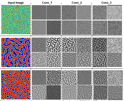
Figure 3.3
Sample response maps in developed CNN for 2D microstructure
morphology inputs. The response map of the first four filters of three convolutional
layers is illustrated for three input images. The layer numbers are presented at the
top of the images.
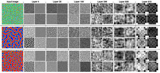
Figure 3.4
Sample response maps in EfficientNetB7 for 2D microstructure morphology
inputs. The response map of the first four filters of some convolutional layers is illustrated
for three input images. The layer numbers are presented at the top of the images.
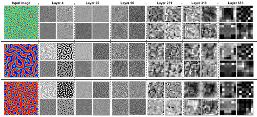
Figure 3.5
Sample response maps in EfficientNetB6 with 2D microstructure
inputs. The response map of the first four filters of some convolutional layers is
illustrated for three input images. The layer number is presented at the top of the
figure.
The response maps for both trained CNN and pretrained EfficientNet show that the first layers capture the simple features like edges, colors, and orientations, while the deeper layers extract more complicated features that are less visually interpretable, see Figure 3.4; similar observations are reported in other studies [65, 67, 177]. The filters from the first layers can extensively detect the edges; hence the microstructures are segmented by the borders of two different phases. By going into deeper layers, understanding the extracted information by the filters becomes more difficult and can only be analyzed by their effects on the accuracy of the final model. Since the pretrained EfficientNet has deeper layers, they can extract more complicated features from the micro structure morphologies. Indeed, we can use different layers for micro structure
information extraction and test them to predict the processing history and find the most optimum network.
Temperature and Chemical Compositions Prediction
The mixed dataset contains microstructure morphologies as image data and the minimum and maximum of Fe composition in the microstructures as numeric data. The most common reported experimental images in literature for the spinodally decomposed microstructures are greyscale TEM images. To enable the model to predict the chemistry and processing history of the experimental microstructures, we have used the greyscale images in the network training. The proposed CNN, as well as EfficientNet-B6 and EfficientNet-B7 pretrained networks, were used for microstructures’ feature extraction.
Then, the extracted features are passed through the fully-connected layers with batch normalization, Swish activation function, and dropout. The numeric data was proceeded by fully-connected layers with the ReLU activation function. The output of both layers was combined with other fully-connected layers to predict temperature and chemical compositions through the linear activation in the last fully-connected layer. After testing different fully-connected layer sizes, the best architecture was selected based on prediction accuracy and stability, which is shown in Figure 2.2 for the proposed CNN and Figure 3.6 for pretrained networks. The models were trained on XSEDE resources [178]. As a starting point, the proposed CNN network with fully-connected layers was trained to predict the processing history parameters. After testing different CNN architectures, the presented network in Figure 2.2, provided the best results that are given in Figure 3.7. The results show that the proposed network can predict the chemical compositions reasonably well, but the temperature accuracy is poor. Temperature is a key parameter in the spinodal decomposition process and developing a model with higher accuracy is required. To increase the accuracy, we need to extract more subtle features from the morphologies. However, training a CNN with more layers requires numerous training data.
A pretrained network can extract more valuable features from images and consequently can be helpful for accuracy improvement. Therefore, after fixing the architecture of fully-connected layers, different layers of EfficientNet-B6 and EfficientNet-B7 were tested to find the best layer for microstructures’ feature extraction. Herein, layers 96, 111, 142, 231, 304, 319, 362, 392, 496, 556, 631, 659, and 663 from EfficientNet-B6 and layers 25, 108, 212, 286, 346, 406, 464, 509, 613, 673, 806, and 810 from EfficientNet-B7 were selected to quantify the microstructures. The models were run, based on the given parameters in Table 2.4, for different layers. The model training was repeated five times. The average R Squares and mean square error (MSE) for cross validation and test set are given in supplementary materials, Table 3.1 and Table 3.2, for EfficientNet-B6 and EfficientNet-B7, respectively. Indeed, the models were validated by 5-fold cross-validation during training, and the test set contains the data that the model never sees in the training process. According to the results, both trained models based on EfficientNet-B6 and EfficientNet-B7 can predict the Co composition very well and while the prediction of temperature and Cr composition is good, they are more challenging. Accordingly, the most accurate prediction belongs to the models that use up to layer 319 of the EfficientNet-B6 and layer 806 of EfficientNet-B7 for microstructures’ quantification.
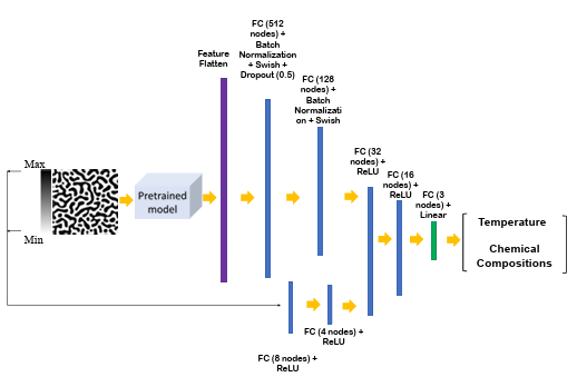
Figure 3.6
The architecture of the proposed model (input image size is 224 × 224
pixels).
In addition to cross-validation and test set accuracy, which can be used for over fitting identification, tracking the loss change in each epoch during the training process can also help in over fitting detection. Figure 3.8a depicts the loss change in each epoch for the developed model based on Efficient Net-B7, a corresponding plot for Efficient Net-B6 is available in supplementary materials, Figure 3.9a. Figure 3.8a shows that both training and validation losses reduce smoothly with the epoch increase. The insignificant gap between the train and validation losses proves that the models’ parameters converge to the optimal values without over fitting. To better understand the application of the developed models, the models were tested by a sample from the test set; the micro structure belongs to the spinodal decomposition of 20% Fe, 40% Cr, and 40% Co at 913 K after 100 hr. The model predictions for temperature and chemical compositions are given in Figure 3.8b, for EfficientNet-B7, and Figure 3.9b, for EfficientNet-B6. The comparison between the ground truth and prediction demonstrates that the models can predict the chemistry and processing history reasonably well.
To quantify the models’ predictive accuracy on all test data points, we have used the parity plots in which the models’ predictions are compared with ground truth in an x-y coordinate system. For an ideal 100% accurate model all data points will overlap on a 45 degree line. The parity plots of the models, i.e., EfficientNet-B7 and EfficientNet-B6, for temperature, Cr composition, and Co composition along with their accuracy parameters are given in Figure 3.8c and Figure 3.9c. The results show that the models can predict the Co composition with the highest accuracy. It seems that temperature prediction is the most challenging variable for the models, but still, there is a good agreement between the models’ prediction and ground truth.
Table 3.1 R-squared and MSE of model predictions for training and testing dataset when different layers of EfficientNet-B6 are used for microstructures’ feature extraction.
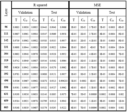
Table 3.2 R-squared and MSE of model predictions for training and testing dataset when different layers of EfficientNet-B7 are used for microstructures’ feature extraction.


Figure 3.7a) Training and validation loss per each epoch, b) prediction of temperature and chemical compositions for a test dataset, and c) the parity plots of temperature and chemical compositions for the testing dataset from the proposed model when proposed CNN are used for micro structures’ feature extraction (input image size is 224 × 224 pixels)
The results include two important points. First, while the extracted features from the shallow trained CNN can predict the compositions well, we need deep CNN to precisely predict the temperature. For this reason, the deep pretrained EfficientNet networks were used, which could predict temperature with higher accuracy. This observation indicates that the compositions are more relevant to simple extracted features of the microstructure morphology, however, more complicated extracted features are required to estimate the temperature. The physical concepts of the problem can also explain this. A small change in compositions would alter the microstructure morphology much more dramatically than a small change in temperature.
The differences among the microstructures with different compositions and the same processing temperature are easily recognizable. For example, with a slight change in chemistry the volume fraction of the decomposed phases would vary and this information, i.e., change in the number of white and black pixels, can easily get extracted from the very first layers of the network. However, there are subtle differences between the microstructure morphologies when we slightly change the processing temperature. Therefore, much more complex features are needed to distinguish the differences among the morphologies with small processing temperature variations. Extraction of these complex features requires deeper convolutional layers. In addition, with convolutional layers increasing, the receptive field size would improve. And that ensures no important information is left out from the microstructure when making predictions. Therefore, more information is extracted from the microstructures, and it would also increase the temperature prediction accuracy. On the other hand, training a deep CNN with limited training and test dataset is not practical. To overcome this challenge, transfer learning can be helpful, and some other studies have shown that pretrained networks are effective in feature extraction in materials science related micrographs [25, 36, 52, 72, 179-181].
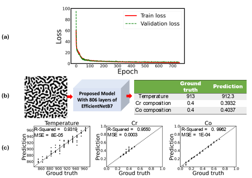
Figure 3.8 a) Training and validation loss per each epoch, b) prediction of temperature and chemical compositions for a random test dataset, and c) the parity plots of temperature and chemical compositions for the testing dataset from the
proposed model when first 806 layers of EfficientNetB7 are used for microstructures’ feature extraction (The size of the input images are 224 × 224 pixels)
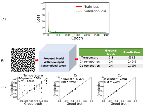
Figure 3.9 a) Training and validation loss per each epoch, b) prediction of temperature and chemical compositions for a test dataset, and c) the parity plots of temperature and chemical compositions for the testing dataset from the proposed model when proposed CNN are used for microstructures’ feature extraction (input image size is 224 × 224 pixels)
Validation of The Proposed Model with The Experimental Data
The model accuracy against the test dataset, i.e., the data that the model has never seen in the training process, is good, but the test dataset is still from phase-field simulation. Since the ultimate goal of the developed framework is to facilitate the micro structure mediated materials design via predicting chemistry and processing history for experimental micro structures, it is valuable to test the model accuracy on the real micro structures. For this purpose, we have tested the model against an experimental TEM image for spinodal decomposition of Fe-Cr-Co with initial composition 46% Fe, 31% Cr, and 23% Co after 100 hr heat treatment at 873 K from Okada et al. [182]. Since the Fe composition of the micrograph was not reported in Okada et al.’s paper, we selected the Fe composition by interpolating between the adjacent simulation points in our database. Figure 3.10 shows the predictions of the proposed network for an experimental TEM micro structure.
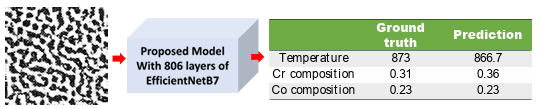
Figure 3.10 Prediction of chemistry and processing temperature for an experimental TEM image adopted from Okada et al. [182]. The original image was cropped to be in the desired size of 224 × 224 pixels.
While Co composition and processing temperature prediction is very good, we see a 16% error in Cr composition prediction. We believe the error could stem from several factors. Firstly, the TEM micrograph that we used does not have the image quality of the training dataset. Secondly, the Fe composition associated with the micrograph was not reported in the original paper [182], and we used a phase-field-informed Fe composition. Thirdly, the dimension of the experimental image was larger than the simulated data, and it was cropped to be at the same size as the required input microstructure size. Despite all these limitations, the proposed model based on the first 806 convolutional layers of Efficient NetB7 predicts the chemistry and processing temperature of an experimental TEM image reasonably well. And it demonstrates that the developed model in this work is suitable for finding the process history behind the experimental micro structures.
Beyond the specific model alloy that we used in this work, the developed model can also be generalized to other materials by considering the material production processes. The developed framework can be used for other ternary alloys that are produced by spinodal decomposition. The model performance in the process history and chemistry prediction should be considered for other spinodal decomposed alloys with less or more elements. The domain adaptation methods such as unsupervised domain adaptation [183] can provide the ability to use the developed model for other spinodal decomposed alloys. In practice, the proposed model needs two experimental inputs, 1) a TEM micrograph that shows the morphology and, 2) X-ray fluorescence spectroscopy (XRF) that provides the corresponding compositions.
Conclusion
We introduced a framework based on a deep neural network to predict the chemistry and processing history from the materials’ microstructure morphologies in this chapter. As a case study, we generated the training and test dataset from phase-field modeling of the spinodal decomposition process of Fe-Cr-Co alloy. We considered a mixed input dataset by combining the image data, the produced micro structure morphologies based on Fe composition, with numeric data, the minimum and maximum of Fe composition in the microstructure. The temperature and chemical compositions
were predicted as processing history. We quantified the micro structures by a proposed CNN and different convolutional layers of EfficientNet-B6 and EfficientNet-B7 pretrained networks. Then, the produced features were combined with the output of a fully-connected layer for numeric data processing by other fully-connected layers to predict processing history.
After testing different architectures, the best network was found based on the model’s accuracy. A detailed analysis of the model’s performance indicated that the model parameters were optimized based on training and validation loss reduction. The results show that while the simple extracted features from the microstructure morphology by the first convolutional layers are enough for the chemistry prediction, the temperature needs more complicated features that can be extracted by deeper layers. The model benchmark against an experimental TEM micrograph indicates the model’s well predictive accuracy for real alloy systems. We demonstrated that the pretrained convolutional layers of EfficientNet networks could be used to extract the meaningful features relevant to the compositions and temperature from the microstructure morphology. In general, the proposed models were able to predict the processing history based on the materials’ microstructure reasonably well.
Data availability
The raw/processed data and codes required to reproduce these findings are available at https://github.com/Amir1361/Materials_Design_by_ML_DL.
CHAPTER FOUR: PROCESSING TIME, TEMPERATURE, AND INITIAL CHEMICAL COMPOSITION PREDICTION FROM MATERIALS MICROSTRUCTURE BY DEEP NETWORK FOR MULTIPLE INPUTS AND FUSED DATA
In this chapter, we consider heat treatment time as another processing parameter for process history and chemistry prediction from materials microstructure.
The result provided in this chapter is published as a research paper [184] in the
Materials & Design Journal (Volume 219, July 2022, 110799,
https://doi.org/10.1016/j.matdes.2022.110799).
Phase-Field Modeling and Dataset Generation
We ran the PF model for the different combinations of time, temperature, and chemical compositions informed by the Simplex-Lattice design. Within the ranges given in Table 2.3, 125,233 different samples were simulated by the PF method, and the microstructures were extracted for different chemical compositions, temperatures, and time. Figure 4.1 depicts the sample results of the PF simulation. MOOSE simulations of the 2D domains take approximately 120 service units (SU) per run on a 24 Core CPU. Therefore, screening the proposed range of different temperatures and chemical compositions for microstructure evolution required approximately 505k SU to complete.
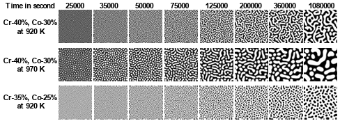
Figure 4.1
The phase-field method generates Fe-Cr-Co alloy microstructures
(Compositions are in atomic percent).
Since decomposition does not occur for all proposed operating conditions and chemistries, the microstructures showing the 0.1 difference in Fe composition between Cr-rich and Fe-rich phases and at least 15 % volume fraction for each phase were considered as spinodally decomposed results. Hence, only 14,376 samples in which decomposition has taken place are used to create the database. 80% of samples were used for training and 20% for testing. The training was validated by 5-fold cross-validation. The Fe-based composition microstructure morphologies, as well as minimum and maximum of Fe compositions in the microstructure along with corresponding time, temperature, and chemical compositions, form the dataset. A sample workflow of the dataset construction is given in Figure 4.2.
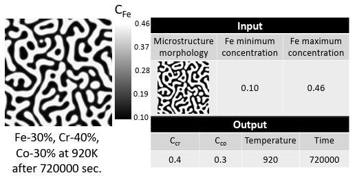
Figure 4.2
A sample workflow of dataset construction.
Deep Network Training
First, the in-house CNNs with different convolutional layers have been tested to find the best architecture. The results are given in Table 4.1. The results indicate that the CNNs can predict the chemistry reasonably well. The accuracy of time prediction increases proportionally with the number of filters. However, the temperature accuracy is poor for all networks. According to previous study findings [185], the temperature is related to complicated microstructure features that can only be extracted by deep convolutional layers. Training such a deep network needs a very large training dataset, which is not available. Therefore, we adopted the transfer learning method to check the network accuracy. We used the Efficient Net-B7 convolutional layers to extract the salient features of the produced microstructure by the PF method as transfer learning. The Efficient Net-B7 has 66 million parameters which are less than other networks with similar accuracies, such as VGG16, etc. Similar to other studies [65, 67, 177], the first layers capture simple features like edges, colors, and orientations. In contrast, the deeper layers extract more complicated, less visually interpretable features (see Figure 4.3).
The fused data, including microstructure morphology and Fe minimum and maximum concentration in morphology, are used for network training. Different pretrained convolutional layers of EfficientNet-B7 are applied to extract micro structures salient features while numeric data is proceeded by fully-connected layers. After passing fully connected layers, the extracted features by convolutional layers are combined with the numeric data through the fully-connected layers to predict the outputs by linear activation function in the last layer, see Figure 4.4. Convolutional layers 25, 108, 212, 286, 346, 406, 464, 509, 613, 673, 806, and 810 from EfficientNet-B7 are used to extract the micro structures features. For different convolutional layers, the model is trained based on the given parameters in Table 2.4.
The model training is based on 5-fold cross-validation and dividing the dataset into training (80%) and testing (20%) datasets. The average R Squares and mean square error (MSE) for cross-validation and test set that the model never sees in the training process are given in Table 4.2. According to the results, the prediction of time and temperature is more challenging than compositions. Almost all the models can predict the compositions very well. The whole training process was repeated three times to check the models’ stability. Finally, the most accurate prediction belongs to the model that uses up to layer 286 of the EfficientNet-B7 for micro structures’ quantification. The error distribution of this model, which shows a normal distribution, is given in Figure 4.5.
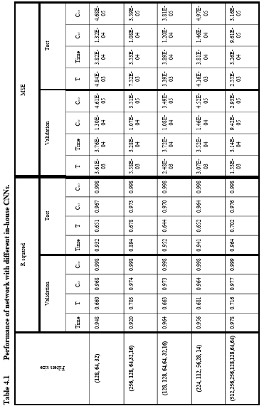
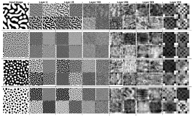
Figure 4.3 Sample response maps in Efficient NetB7 with 2D micro structure inputs. The response map of the first four filters of some convolutional layers is illustrated for four input images. The layer number is presented at the top of the figure.
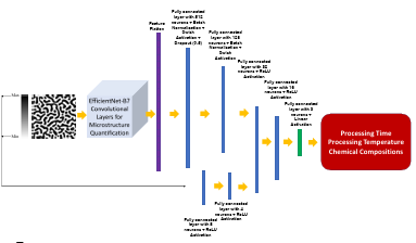
Figure 4.4
The architecture of the proposed model (input image size is 224 × 224 pixels).
In addition to cross-validation, testing data has also been used for overfitting detection. The training and validation losses diminish smoothly with epoch, as shown in Figure 4.6a, and it is an indication that the model parameters converge to the global optimum without overfitting. A sample from the test set is given in Figure 4.6b to show the developed model performance. The presented microstructure is for 15% Fe, 25% Cr, and 60% Co (all in atomic percent) after 195000 seconds of heat treatment at 950 K. The model’s predictions have good agreement with ground truth values for time, temperature,
and chemical compositions. The parity plots with accuracy metrics for comparing the model prediction with ground truth for all testing data are shown in Figure 4.6c. The results show that the model can predict the chemical compositions with the highest accuracy. The prediction accuracy for time and temperature is not as good as chemical compositions. But the model can still predict them reasonably well.
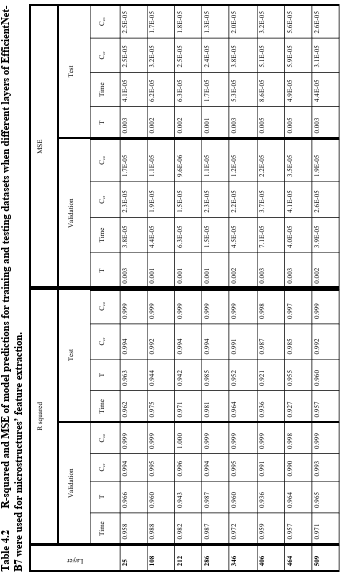
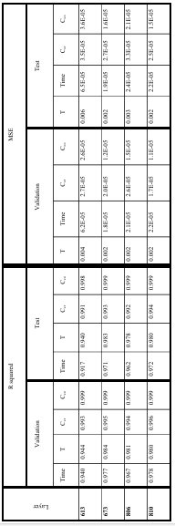
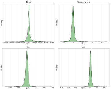
Figure 4.5
Error distribution for the testing dataset from the proposed model
when the first 286 layers of EfficientNetB7 are used for microstructures’ feature
extraction (The size of the input images is 224 × 224 pixels)
The results indicate that the time and temperature prediction is more challenging than chemical compositions, which is explainable by physical concepts. According to our simulation results (see Figure 4.7) and reported studies [182, 186], a slight change in initial chemical compositions can lead to a sensible change in microstructure morphology which is even recognizable by human eyes. Therefore, it will be uncomplicated for the model to realize the chemical composition changes. However, small changes in temperature will hardly lead to noticeable changes in the microstructure morphologies
when the time and chemical composition are fixed. Therefore, finding these differences is hard and makes temperature prediction challenging. In the case of time, there are two different conditions. The morphology changes rapidly with time at the early stages of heat treatment, but the rate of change drops dramatically after some time, i.e., when the
morphology reaches some stability, and changes will be minimal over time. This insensitivity will make the identification strenuous for the model. According to Table 4.2, the models can predict the chemical composition, temperature, and time in order of maximum to least accuracy. However, as we will discuss in the next section, most errors in time and temperatures, are not actually real errors, but just other right answers.
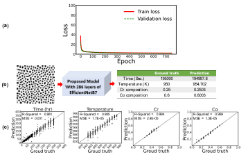
Figure 4.6 a) Training and validation loss per each epoch, b) prediction of time, temperature, and chemical compositions for a random test dataset, and c) the parity plots for time, temperature, and chemical compositions for the testing dataset based on the transfer learning model when the first 286 layers of EfficientNetB7 are used for microstructures’ feature extraction (The size of the input images are 224 × 224 pixels)
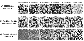
Figure 4.7 Different microstructures a) at constant time and temperature, b) at constant time and chemical compositions, and c) at constant temperature and chemical compositions.
Model Performance Analysis
The R-square and RSME results for testing points show that the model can predict time, temperature, and chemical compositions well. However, the model’s reliability depends on knowing the sources of the errors. Therefore, in this section, we will do a more in-depth study on some low-accuracy cases to find out the source of errors. As was mentioned earlier and according to the parity plots in Figure 4.6c, the lowest accuracy belongs to time and temperature predictions. Some worst cases in time and temperature prediction are given in Figure 4.8.
After studying some random cases, among the predictions with high errors, we concluded that two scenarios are possible for the sources of errors. One is achieving stability in the microstructure morphology after a certain time, and the second is achieving an identical microstructure from two different paths. Based on the observations and physical concepts, the microstructure morphologies change very sluggishly with time after passing the early stages of separation and coarsening, and reach some sort of stability.
As mentioned earlier, once the stability is achieved, it is hard for the model to distinguish the differences between the microstructures due to the subtle or no changes between two considerable time steps. Therefore, we hypothesize that the errors that we observe in time predictions for high heat treatment times, i.e., times above 100 hrs, are associated with morphology stability. To test this hypothesis, we compared the simulated microstructures based on the model’s predictions with the microstructure given as the input, i.e., ground truth, to the modal.
Quantitative comparison of different images can be made either by evaluating specific metrics or by observing the distribution of defined parameters in the images. We adopted some evaluation metrics that were widely used in the computer vision community including the Root Mean Squared Error (RMSE), Peak Signal-to-Noise Ratio (PSNR) [187, 188], the Structural Similarity Index Measure (SSIM) [189], and the Learned Perceptual Image Patch Similarity (LPIPS) [158]. In these metrics, smaller RMSE and LPIPS, and higher PSNR and SSIM indicate more similarity between images. For distributions comparison between two images, two-point correlation function [160] and chord length [161] are standard techniques and we used them in this study. Figure 4.9 shows the comparison between the ground truth and simulated
microstructure for the first row of Figure 4.8.
We note that the simulated microstructures in Figure 4.9 are informed by the DL-predicted chemistry, temperature, and time, i.e., the prediction values in Figure 4.8. The evaluation metrics and distributions demonstrate that the two microstructures are similar, while there is about 70 hrs differences in their heat treatment times. These quantitative comparisons endorsed our hypothesis that the errors that we observe in time predictions for high heat treatment times are associated with the morphology stability.
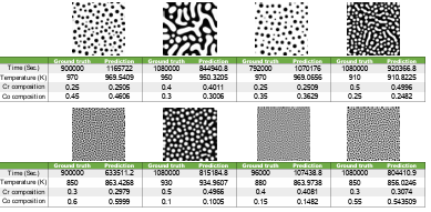
Figure 4.8
Some worst cases for time (first row of images) and temperature (second row of images) predictions.

Figure 4.9 Comparison of the ground truth microstructures with the simulated microstructures from model predictions for four random cases with high errors in time.
Another source of error that we observed in predictions stems from the interplay between time and temperature. For these types of errors, we hypothesize that the predicted processing conditions, while being different from the ground truth, are indeed another path to reach a similar microstructure. To test this hypothesis, we ran the PF model with the predicted chemistry and processing parameters and compared quantitatively the simulated microstructures with the ground truth microstructures in Figure 4.10. Again, the metrics and distributions show that the microstructures are very similar, and in fact, we can generate similar microstructures from two separate paths, i.e., higher time/lower temperature and lower time/higher temperature. Therefore, in these cases, the model does not predict wrong processing but just discovers a new path.
Therefore, according to the model review results, the primary sources of errors, primarily in heat treatment time and temperature, root in the physical concepts behind the spinodal decomposition and are not inherently wrong predictions but just another right answer.
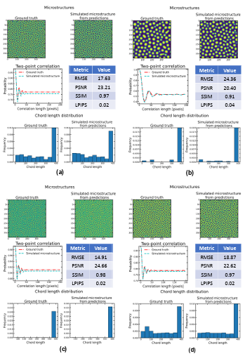
Figure 4.10 Comparison of the ground truth microstructures with the simulated microstructures from model predictions for four random cases with errors in time and temperature.
Validation of The Proposed Model with the Experimental Data
The main motivation of the proposed model is to enable the chemistry and processing history prediction of a micrograph. This makes the model a unique tool that enables, for the first-time, microstructure inverse design possible with no lost information, i.e., reducing the complexity of microstructure to just average grain size, etc. Since ultimately, the predicted chemistry and processing parameters are going to feed into the experiment, the model validation is crucial. In this section, we validate the model’s predictability against an experimental transmission electron microscopy (TEM)
image for spinodal decomposition of Fe-Cr-Co with the initial composition of 46% Fe, 31% Cr, and 23% Co after 100 hrs of heat treatment at 873 K from Okada et al. [182]. The original TEM image was larger than the model’s required input size, so it was cropped to meet the 224×224 pixels size. Also, the Fe composition minimum and maximum in the micrograph were not given, and we selected these values by interpolating between the adjacent simulation points in the database. Figure 4.11 Figure 3.10shows the predictions of the model for the experimental TEM microstructure along with the ground truth.

Figure 4.11 Prediction of processing time, temperature, and chemistry for an experimental TEM image adopted from Okada et al. [182]. The original image was cropped to be in the desired size of 224 × 224 pixels.
Comparison between the predicted and ground truth shows that the model performs very well in terms of Co composition and temperature predictions with just 0.6% and 0.9% error, respectively. The predictions show 10% and 15% errors for annealing time and Cr composition, respectively. While all computational models naturally have some errors, we identify five key sources for the uncertainties in using the model for experimental micrographs, 1) the TEM micrograph does not have the image quality of the simulation microstructures, i.e., the training data, 2) the TEM image size was larger than the model’s input, and we cropped it to 224×224 pixels, 3) the Fe composition was not reported for the TEM image and we used the PF input, 4) the model was trained with synthetic data and not TEM micrographs, 5) the PF model was parameterized with CALPHAD, and some errors correlate with uncertainty in CALPHAD data. These uncertainties can be reduced if there are enough experimental images to be used in the training dataset. Despite all these shortcomings, the model’s predictions for chemistry and processing history for the TEM micrograph were reasonably well.
Conclusion
In this chapter, we have developed a computational framework that enables the microstructure inverse design. As a model material, we studied the Fe-Cr-Co based permanent magnet alloys. The developed deep neural network is able to read a
micrograph of one element distribution and predicts the chemistry and processing parameters that would lead to that micrograph. The model integrates the physics-based and data-driven modeling. The training and testing data were generated from the phase field modeling of the spinodal decomposition process in Fe-Cr-Co alloys. The fused input data, including the microstructure morphologies and the associated minimum and maximum Fe composition, were used to train the proposed network to predict the heat treatment time and temperature as well as the initial chemical composition, i.e., the Cr and Co.
We used different CNN layers as well as different convolutional layers of EfficientNet-B7 pretrained networks to quantify the microstructure morphologies. The accuracy metrics, parity plots, and error distribution demonstrate that the model with the EfficientNet-B7 pretrained network performs well on the training data. We found that temperature is the most challenging parameter to predict and it requires deeper layers and more complicated extracted features from micro structures. The error analysis showed that some wrong predictions, in particular the ones with high errors in time and temperature predictions, are not actually wrong but just other correct answers. We identified that the errors are associated with either the microstructure morphology stability or the possibility of having one microstructure with two processing paths. Finally, we validated the model with an experimental TEM microstructure and the model was able to predict the
processing history and chemistry of the TEM micrograph reasonably well.
The process parameters and chemistry prediction for experimental micrographs can improve significantly if we have the right size, and high-resolution micro structures, and also add some experimental data to the training dataset.
Data availability
The raw/processed data and codes required to reproduce these findings are available at
https://github.com/Amir1361/time_temperature_composition_predictionhttps://github.co
m/Amir1361/Materials_Design_by_ML_DL.
CHAPTER FIVE: SPATIOTEMPORAL PREDICTION OF MICROSTRUCTURE EVOLUTION WITH PREDICTIVE RECURRENT NEURAL NETWORK
In this chapter, we propose a Predictive Recurrent Neural Network (PredRNN) model for microstructure evolution prediction, which extends the inner-layer transition function of memory states in LSTMs to spatiotemporal memory flow.
The result provided in this chapter is submitted as a research paper in the Materials & Design Journal (October 2022).
Phase-Field Modeling for Micro structure Sequences Generation
Following the Simplex-Lattice design, the microstructure sequences are produced by PF modeling Fe-Cr-Cr spinodal decomposition for the different times, chemical compositions, and temperatures. The microstructures were retrieved for 125,233 different samples that were simulated using the PF approach within the parameters listed in Table 2.3 for various chemical compositions, temperatures, and times. The sample micro structure sequences from PF simulation results are shown in Figure 4.1. On a 24 Core CPU, a MOOSE simulation of the 2D domains uses about 120 service units (SU) every run.
Therefore, it took around 505k SU to screen the suggested range of various temperatures and chemical compositions for microstructure evolution. In other words, each MOOSE simulation of a 200 nanometer 2D domains takes approximately 120 hrs per run for 100 mesh grid on a 24 Core CPU. Figure 4.1 indicates that the micro structure evolution process differs in various chemical compositions and temperatures. The training dataset can be generated from simulated micro structures. The length of each sequence is 20 microstructures. The first 10 microstructures are for the first 30 hr of heat treatment time and are used to predict the future 10 microstructures, which belong to 50 hr to 300 hr, as output sequence. There are 20,000 sequences for training and 4,000 sequences as testing data. Three different Fe-composition-based micro structure morphology sequences are presented in Figure 5.1.
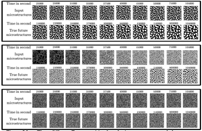
Figure 5.1
Three different Fe-composition-based microstructure morphology sequences
As can be seen, the dataset contains very different evolution sequences in terms of structure. In addition, since the microstructures are selected from both distinct stages of spinodal decomposition, a fast composition modulation growth stage and a slower coarsening stage, the difference between the input and output sequence is significant, which can be easily recognized in Figure 5.1. In this case, the model has a more difficult task in predicting the output sequence.
Microstructure Evolution Prediction by PredRNN
20,000 sequences trained the PredRNN to predict the output micro structures. With a mini-batch of 8 sequences, we trained the models using the ADAM optimizer. After 80,000 iterations, the training process is terminated with a learning rate of 10-4. PredRNN typically employs four ST-LSTM layers to balance training effectiveness with prediction quality. We set the size of the convolutional kernels inside the ST-LSTM unit to 5×5 and the number of channels of each hidden state to 128. As illustrated in Figure 5.2, the training loss decreases smoothly with iteration, which indicates that the model’s parameters have reached their optimal value globally. In addition, we employ evaluation measures that are frequently used to determine how similar two images are.
The predicted and ground truth microstructures are compared using the Mean Squared Error (MSE), the peak signal to-noise ratio (PSNR), the Structural Similarity Index Measure (SSIM), and the Learned Perceptual Image Patch Similarity (LPIPS). The distinction between these metrics is that PSNR compares image compression quality, SSIM measures the similarity of structural information within the spatial neighborhoods, and LPIPS is based on deep features and is more in line with human perceptions. MSE estimates the absolute pixel-wise errors. Smaller MSE and LPIPS, and higher PSNR and SSIM indicate more similarity between images.
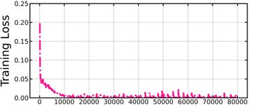
Figure 5.2 Training loss per iteration
After training, test sequences are used to compute MSE, LPIPS, PSNR, and SSIM; the average values for each iteration are given in Figure 5.3. The results demonstrate that all the metrics improve with iteration to reach almost stability. It proves that the model learns from the data and can train the hyper parameters.
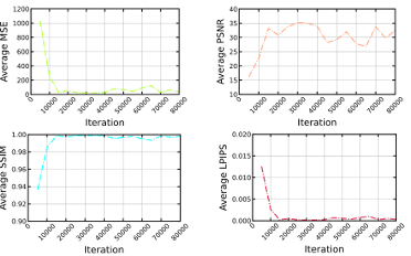
Figure 5.3
Average MSE, PSNR, SSIM, and LPIPS for test sequences during training per each iteration
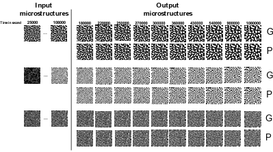
Figure 5.4 Frame-wise results on the three randomly selected samples from the test set produced by the final PredRNN model (predictions (P) vs. ground truth (G))
Figure 5.4 displays three randomly selected samples from the test set for a qualitative comparison. The left microstructures of the dashed line are the input frames, the right ones in the top row are the ground truth of output microstructures, and the bottom row shows the PredRNN prediction. The microstructures produced by PredRNN predict clear images, meaning it can be confident of future variations. In addition, we can see that the predicted sequence is close to the ground truth sequence.
Trained Model Performance on The Microstructure Evolution Prediction During Time
Model performance frames prediction during time is one of the key parameters in spatiotemporal models’ evaluation [190, 191]. Basically, the perdition of earlier frames because of similarity with input sequence is easier than long-term prediction. Figure 5.5 provides the corresponding frame-wise comparisons between the final PredRNN model predictions and ground truth microstructures for test sequences. The average values of metrics show that the model can predict all the microstructures with reasonable accuracy. On the other hand, the model is more powerful in predicting the first frames than the last as MSE and LPIPS increase and PSNR and SSIM decrease from time step 1 to 10. For qualitative comparison of long-term and short-term prediction, three randomly selected samples from the test set produced by the final PredRNN model are given in Figure 5.6. The results show that PredRNN prediction for short-term cases is more accurate than long-term prediction. These results seem reasonable because there is a stronger relationship between the first microstructure from the output sequence and the input sequence. However, in general, the predictions for long-term cases also have good agreement with the ground truth. It proves that the PredRNN can predict the micro structure evolution reasonably well.
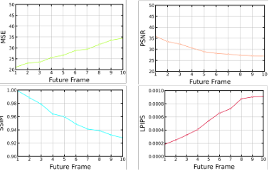
Figure 5.5 Frame-wise results on the test set produced by final PredRNN model
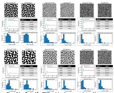
Figure 5.6 Trained PredRNN model performance on short and long-term prediction for three randomly selected samples from the test set
Trained Model Inference Performance in Future Microstructures Prediction
The time it takes to calculate the model’s outputs as a function of the inputs is known as the inference speed. The model’s response time is crucial in many applications, especially those requiring real-time data [192]. Since this study aims to develop a deep network to predict the microstructure evolution quickly and accurately, the model inference performance is a principal factor. Therefore, the trained model performance is compared with the simulation on a reference computer. Since MOOSE can only run with the CPU, we used the same resource for the trained model. The result for randomly selected test data is given in Figure 5.7. While the simulation of rest microstructures takes more than 75 hr by PF modeling, the trained model can predict the future sequence quickly by just having earlier microstructures. The error metrics indicate that this prediction is robust and reliable compared to simulated microstructures.
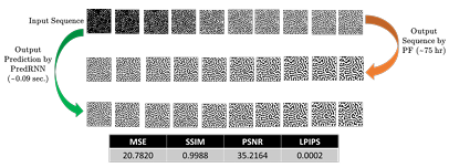
Figure 5.7 Comparison of trained PredRNN model speed with PF simulation on a randomly selected sample from the test set
Conclusion
We introduced a framework based on a deep neural network to predict the material microstructure evolution. As a case study, we generated the training and test dataset from phase-field modeling of the spinodal decomposition process of Fe-Cr-Co alloy. We considered the microstructure morphologies evolution based on Fe composition. The future microstructure sequence was predicted by knowing the earlier sequence by PredRNN. A detailed analysis of the model’s performance indicated that the model parameters were optimized based on training loss reduction and error metrics improvement. The quantitative and qualitative comparisons show that the trained PredRNN model can predict the output sequence accurately. Although the model accuracy for the short-term prediction is better than the long-term prediction, the model still shows reliable performance in the long-term forecasting. The model inference test demonstrates that it can predict the microstructure evolution quickly and accurately. In general, the proposed models could reasonably predict the materials’ microstructure evolution.
Data availability
The trained model parameters and dataset to reproduce these findings are available at https://doi.org/10.24435/materialscloud:es-a4
CONCLUSION AND FUTURE WORKS
This dissertation aims to present using the deep neural network on the materials’ microstructure that plays a critical role in the properties and performance of materials. This dissertation attempts to achieve these research goals based on the following steps. A deep neural network for chemical compositions and process history in steady state processes was developed at the first step. While the simulation methods based on physical concepts, such as the PF method, can predict the spatiotemporal evolution of the materials’ microstructures, they are not efficient techniques for predicting processing and chemistry if a specific morphology is desired. The model alloy used in this work is Fe Cr-Co permanent magnets. These alloys experience spinodal decomposition at temperatures around 850 – 970 K. We used the PF method to create the training and test dataset for the DL network. The PF results are extracted after the 100 hr spinodal decomposition process, and all the training data are independent of time. The mixed dataset, which includes both images, i.e., the morphology of Fe distribution, and continuous data, i.e., the Fe minimum and maximum concentration in the microstructures, are used as input data, and the spinodal temperature and initial chemical composition are utilized as the output data to train the proposed deep neural network. A CNN will quantify the produced microstructures by the PF method; then, another deep neural network will use the salient features to predict the temperature and chemical composition. The proposed convolutional layers were compared with pretrained Efficient Net convolutional layers as transfer learning in micro structure feature extraction.
We quantified the microstructures by using a suggested CNN and various convolutional layers of the pretrained EfficientNet-B6 and EfficientNet-B7 networks. Then, further fully-connected layers integrated the generated features with the output of a fully connected layer for processing numerical data to forecast processing history. The most accurate network was discovered after evaluating various microstructures. A thorough examination of the model’s performance revealed that the model’s parameters were chosen to minimize loss during training and validation. The findings demonstrate that while the chemistry prediction may be made with just the basic elements that were derived from the microstructure morphology by the first convolutional layers, the temperature prediction requires more sophisticated data that deeper layers can extract.
The model’s comparison to an experimental TEM micrograph shows that it is highly accurate in predicting the behavior of real alloy systems. We showed that the meaningful information pertinent to the compositions and temperature could be extracted from the microstructure morphology using the pretrained convolutional layers of EfficientNet networks. Generally speaking, the proposed models were able to fairly accurately predict the processing history based on the microstructure of the materials.
As mentioned, prediction of the chemical composition and processing history from microstructure morphology can help optimize processing conditions and discover possible processing paths for a targeted microstructure. But we did not consider the process treatment time effect on the microstructures in the first step. In the second step, we proposed a deep learning framework that can predict the treatment time, temperature, and chemistry of a microstructure just by knowing the morphological distribution of one element. We again used the Fe-Cr-Co-based permanent magnet alloy as model material.
We generated a dataset by simulating the spinodal decomposition process in Fe-Cr-Co alloys using the PF method. In this case study, the time, temperature, and initial chemical compositions are used as output, i.e., processing history, while the mixed dataset of microstructure morphology, as image data, and minimum/maximum of iron concentration in the morphology as numeric data are input.
To characterize the microstructure morphologies, we used several CNN layers as well as various convolutional layers of EfficientNet-B7 pretrained networks. The model with the EfficientNet-B7 pretrained network works well on the training data, as shown by the accuracy metrics, parity plots, and error distribution. We discovered that the most difficult characteristic to predict is temperature, which calls for deeper layers and more intricately derived features from microstructures. The error analysis revealed that some incorrect predictions—particularly those with significant errors in time and temperature predictions—were simply other right responses. We identified that the inaccuracies are related to either the stability of the microstructure morphology or the potential for a single microstructure to have two processing routes. Finally, we tested the model using an experimental TEM microstructure, and the results showed that the model was reasonably accurate in predicting the chemistry and processing history of the TEM micrograph.
If we have the appropriate size and high-resolution microstructures and include some experimental data in the training dataset, the process parameters and chemical prediction for experimental micrographs can be much enhanced. Data set generation in the first two parts of the thesis was very expensive. With the aim to expand the current model to more complex alloys, the data set generation will become a bottleneck. Therefore, in the third step, we presented a deep neural network based framework to predict the materials microstructure evolution, which is a spatiotemporal prediction problem. In this case study, we used PF modeling to create the training and test datasets for the spinodal decomposition of a Fe-Cr-Co alloy. We took into account the evolution of micro structure morphologies dependent on Fe composition.
Knowing the earlier sequence through PredRNN allowed us to anticipate the future microstructure sequence. According to a thorough review of the model’s performance, the model parameters were improved based on training loss reduction and improved error metrics. The trained PredRNN model is capable of properly predicting the output sequence, as shown by the quantitative and qualitative comparisons. Although the model’s accuracy for short-term forecasting is higher than that for long-term forecasting, it nevertheless exhibits dependable performance in the latter. In summary, the developed models in this dissertation will be able to find the process conditions and chemical compositions from an ideal microstructure and predict microstructures without expensive and time-consuming simulations and experiments. Doing so provides the materials science community with knowledge and algorithms that can be used for new materials development with the desired properties.
Future Works
Material informatics is one of the rapidly developing fields. With the development of more powerful models, new rooms are opened for AI use in materials science. This work is the first step in our group toward using deep learning and data science in materials design. In the following, we provide some information about how it is possible to expand this study in the future.
• Expand the model to consider 3D microstructures and predict the process history and chemistry behind them. Data generation will be the first challenge in the 3D model. At the same time, training a deep network that can digest the 3D microstructures will be another interesting problem.
• Unknown parameters in microstructure modeling are another challenge in materials design. Several complex parameters, particularly for multicomponent alloys, such as interfacial energies, diffusion coefficients, and coefficients of the Onsager diffusion matrix, are usually very difficult to measure accurately, either experimentally or computationally, and
therefore not available for many materials. We can hypothesize that these parameters could be predicted from a few sets of experimental microstructures with known processing history by a machine learning model that has been trained by physics-based simulations. Our team has recently succeeded in developing a model for the prediction of Onsager and gradient energy coefficients from microstructure images with machine learning.
• Knowledge of the microstructure of the materials during the manufacturing processes, such as additive manufacturing, can greatly improve the final product quality. Live microstructure prediction based on common simulation techniques is not practical because of computational costs. The PredRNN model can be improved to predict the materials’ microstructure based on chemical compositions, processing conditions, and earlier microstructures quickly and accurately.
REFERENCES
1. Rao, C. and Y. Liu, Three-dimensional convolutional neural network (3D-CNN) for heterogeneous material homogenization. Computational Materials Science, 2020. 184: p. 109850.
2.Chen, L.-Q., Phase-field models for microstructure evolution. Annual review of materials research, 2002. 32(1): p. 113-140.
3.Miyoshi, E., et al., Large-scale phase-field simulation of three-dimensional isotropic grain growth in polycrystalline thin films. Modelling and Simulation in Materials Science and Engineering, 2019. 27(5): p. 054003.
4. Zhao, Y., et al., Phase-field simulation for the evolution of solid/liquid interface front in directional solidification process. Journal of Materials Science & Technology, 2019. 35(6): p. 1044-1052.
5.Stewart, J.A. and R. Dingreville, Microstructure morphology and concentration modulation of nanocomposite thin-films during simulated physical vapor deposition. Acta Materialia, 2020. 188: p. 181-191.
6. Beyerlein, I.J. and A. Hunter, Understanding dislocation mechanics at the mesoscale using phase field dislocation dynamics. Philosophical transactions. Series A, Mathematical, physical, and engineering sciences, 2016. 374(2066): p.
20150166.
7.Elliott, C.M. and B. Stinner, A surface phase field model for two-phase biological membranes. SIAM Journal on Applied Mathematics, 2010. 70(8): p. 2904-2928.
8.Karma, A., D.A. Kessler, and H. Levine, Phase-field model of mode III dynamic fracture. Physical Review Letters, 2001. 87(4): p. 045501.
9.Montes de Oca Zapiain, D., J.A. Stewart, and R. Dingreville, Accelerating phase field-based microstructure evolution predictions via surrogate models trained by machine learning methods. npj Computational Materials, 2021. 7(1): p. 3.
10. Brough, D.B., D. Wheeler, and S.R. Kalidindi, Materials Knowledge Systems in Python—a Data Science Framework for Accelerated Development of Hierarchical Materials. Integrating Materials and Manufacturing Innovation,
2017. 6(1): p. 36-53.
11. Meredig, B., Five High-Impact Research Areas in Machine Learning for Materials Science. Chemistry of Materials, 2019. 31(23): p. 9579-9581.
12. Kalidindi, S.R., et al., Role of materials data science and informatics in accelerated materials innovation. MRS Bulletin, 2016. 41(8): p. 596-602.
13. Voyles, P.M., Informatics and data science in materials microscopy. Current Opinion in Solid State and Materials Science, 2017. 21(3): p. 141-158.
14. Haghighatlari, M., et al., ChemML: A machine learning and informatics program package for the analysis, mining, and modeling of chemical and materials data.
15. WIREs Computational Molecular Science, 2020. 10(4): p. e1458. Kalidindi, S.R. and M.D. Graef, Materials Data Science: Current Status and Future Outlook. Annual Review of Materials Research, 2015. 45(1): p. 171-193.
16. Oweida, T.J., et al., Merging Materials and Data Science: Opportunities, Challenges, and Education in Materials Informatics. MRS Advances, 2020. 5(7): p. 329-346.
17. Kalidindi, S.R., A.J. Medford, and D.L. McDowell, Vision for Data and Informatics in the Future Materials Innovation Ecosystem. JOM, 2016. 68(8): p. 2126-2137.
18.Ramakrishna, S., et al., Materials informatics. Journal of Intelligent Manufacturing, 2019. 30(6): p. 2307-2326.
19. Khosravani, A., A. Cecen, and S.R. Kalidindi, Development of high throughput assays for establishing process-structure-property linkages in multiphase polycrystalline metals: Application to dual-phase steels. Acta Materialia, 2017. 123: p. 5569.
20. Cecen, A., et al., Material structure-property linkages using three-dimensional convolutional neural networks. Acta Materialia, 2018. 146: p. 76-84.
21.Jung, J., et al., An efficient machine learning approach to establish structure property linkages. Computational Materials Science, 2019. 156: p. 17-25.
22.Brough, D.B., et al., Microstructure-based knowledge systems for capturing process-structure evolution linkages. Current Opinion in Solid State and Materials Science, 2017. 21(3): p. 129-140.
23. Whelan, G. and D.L. McDowell, Machine Learning-Enabled Uncertainty Quantification for Modeling Structure–Property Linkages for Fatigue Critical Engineering Alloys Using an ICME Workflow. Integrating Materials and Manufacturing Innovation, 2020. 9(4): p. 376-393.
24. Yabansu, Y.C., et al., Extraction of reduced-order process-structure linkages from phase-field simulations. Acta Materialia, 2017. 124: p. 182-194.
25. Ling, J., et al., Building data-driven models with microstructural images: Generalization and interpretability. Materials Discovery, 2017. 10: p. 19-28.
26. Farizhandi, A.A.K., H. Zhao, and R. Lau, Modeling the change in particle size distribution in a gas-solid fluidized bed due to particle attrition using a hybrid artificial neural network-genetic algorithm approach. Chemical Engineering Science, 2016. 155: p. 210-220.
27. Farizhandi, A.A.K., et al., Evaluation of material properties using planetary ball milling for modeling the change of particle size distribution in a gas-solid fluidized bed using a hybrid artificial neural network-genetic algorithm approach. Chemical Engineering Science, 2020. 215: p. 115469.
28. Farizhandi, A.A.K., et al., Evaluation of carrier size and surface morphology in carrier-based dry powder inhalation by surrogate modeling. Chemical Engineering Science, 2019. 193: p. 144-155.
29. Farizhandi, K. and A. Abbas, Surrogate modeling applications in chemical and biomedical processes, in School of Chemical and Biomedical Engineering(SCBE). 2017, Nanyang Technological University.
30. Farizhandi, A.A.K., M. Alishiri, and R. Lau, Machine learning approach for carrier surface design in carrier-based dry powder inhalation. Computers & Chemical Engineering, 2021: p. 107367.
31. Li, L., et al., Understanding machine-learned density functionals. International Journal of Quantum Chemistry, 2016. 116(11): p. 819-833.
32. Nagai, R., R. Akashi, and O. Sugino, Completing density functional theory by machine learning hidden messages from molecules. npj Computational Materials, 2020. 6(1): p. 43.
33. Snyder, J.C., et al., Finding density functionals with machine learning. Physical Review Letters, 2012. 108(25): p. 253002.
34. Gubernatis, J.E. and T. Lookman, Machine learning in materials design and discovery: Examples from the present and suggestions for the future. Physical Review Materials, 2018. 2(12): p. 120301.
35. Liu, R., et al., A predictive machine learning approach for micro structure optimization and materials design. Sci Rep, 2015. 5: p. 11551.
36. Kautz, E., et al., An image-driven machine learning approach to kinetic modeling of a discontinuous precipitation reaction. Materials Characterization, 2020: p. 110379.
37. Bostanabad, R., et al., Computational microstructure characterization and reconstruction: Review of the state-of-the-art techniques. Progress in Materials Science, 2018. 95: p. 1-41.
38. Agrawal, A. and A. Choudhary, Deep materials informatics: Applications of deep learning in materials science. MRS Communications, 2019. 9(3): p. 779-792.
39. Jha, D., et al., Elemnet: Deep learning the chemistry of materials from only elemental composition. Scientific reports, 2018. 8(1): p. 1-13.
40. Xue, D., et al., An informatics approach to transformation temperatures of NiTi based shape memory alloys. Acta Materialia, 2017. 125: p. 532-541.
41. Meredig, B., et al., Can machine learning identify the next high-temperature superconductor? Examining extrapolation performance for materials discovery. Molecular Systems Design & Engineering, 2018. 3(5): p. 819-825.
42. Meredig, B., et al., Combinatorial screening for new materials in unconstrained composition space with machine learning. Physical Review B, 2014. 89(9): p. 094104.
43. Teichert, G.H. and K. Garikipati, Machine learning materials physics: Surrogate optimization and multi-fidelity algorithms predict precipitate morphology in an alternative to phase field dynamics. Computer Methods in Applied Mechanics and Engineering, 2019. 344: p. 666-693.
44. Pilania, G., et al., Accelerating materials property predictions using machine learning. Scientific reports, 2013. 3(1): p. 1-6.
45. Del Rosario, Z., et al., Assessing the frontier: Active learning, model accuracy, and multi-objective candidate discovery and optimization. The Journal of Chemical Physics, 2020. 153(2): p. 024112.
46. Jha, D., et al., Enhancing materials property prediction by leveraging computational and experimental data using deep transfer learning. Nature communications, 2019. 10(1): p. 1-12.
47. Chen, Y., et al., Deep and low-level feature based attribute learning for person re-identification. Image and Vision Computing, 2018. 79: p. 25-34.
48. Hinton, G.E., To recognize shapes, first learn to generate images. Progress in brain research, 2007. 165: p. 535-547.
49. LeCun, Y., Y. Bengio, and G. Hinton, Deep learning. nature, 2015. 521(7553): p. 436-444.
50. Amodei, D., et al. Deep speech 2: End-to-end speech recognition in english and mandarin. in International conference on machine learning. 2016.
51.Cang, R., et al., Microstructure representation and reconstruction of heterogeneous materials via deep belief network for computational material design. Journal of Mechanical Design, 2017. 139(7).
52. DeCost, B.L., et al., High throughput quantitative metallography for complex microstructures using deep learning: a case study in ultrahigh carbon steel. Microscopy and Microanalysis, 2019. 25(1): p. 21-29.
53. Xie, T. and J.C. Grossman, Crystal graph convolutional neural networks for an accurate and interpretable prediction of material properties. Physical review letters, 2018. 120(14): p. 145301.
54. Ryan, K., J. Lengyel, and M. Shatruk, Crystal Structure Prediction via Deep Learning. Journal of the American Chemical Society, 2018. 140(32): p. 10158 10168.
55. Yang, Z., et al., Deep learning approaches for mining structure-property linkages in high contrast composites from simulation datasets. Computational Materials Science, 2018. 151: p. 278-287.
56. Landi, G., S.R. Niezgoda, and S.R. Kalidindi, Multi-scale modeling of elastic response of three-dimensional voxel-based microstructure datasets using novel DFT-based knowledge systems. Acta Materialia, 2010. 58(7): p. 2716-2725.
Kalidindi, S.R., et al., A novel framework for building materials knowledge systems. Computers, Materials, & Continua, 2010. 17(2): p. 103-125.
58. Fast, T. and S.R. Kalidindi, Formulation and calibration of higher-order elastic localization relationships using the MKS approach. Acta Materialia, 2011. 59(11): p. 4595-4605.
59. Yang, Z., et al., Establishing structure-property localization linkages for elastic deformation of three-dimensional high contrast composites using deep learning approaches. Acta Materialia, 2019. 166: p. 335-345.
60. Liu, R., et al., Machine learning approaches for elastic localization linkages in high-contrast composite materials. Integrating Materials and Manufacturing Innovation, 2015. 4(1): p. 192-208.
61. Liu, R., et al., Context Aware Machine Learning Approaches for Modeling Elastic Localization in Three-Dimensional Composite Microstructures. Integrating Materials and Manufacturing Innovation, 2017. 6(2): p. 160-171.
62. Zhao, Y., et al., Predicting Elastic Properties of Materials from Electronic Charge Density Using 3D Deep Convolutional Neural Networks. The Journal of Physical Chemistry C, 2020. 124(31): p. 17262-17273.
63. Kajita, S., et al., A Universal 3D Voxel Descriptor for Solid-State Material Informatics with Deep Convolutional Neural Networks. Scientific Reports, 2017. 7(1): p. 16991.
64. Simonyan, K. and A. Zisserman, Very deep convolutional networks for large scale image recognition. arXiv preprint arXiv:1409.1556, 2014.
65. Chollet, F. Xception: Deep learning with depthwise separable convolutions. in Proceedings of the IEEE conference on computer vision and pattern recognition. 2017.
66. He, K., et al. Identity mappings in deep residual networks. in European conference on computer vision. 2016. Springer.
67. Szegedy, C., et al. Rethinking the inception architecture for computer vision. in Proceedings of the IEEE conference on computer vision and pattern recognition. 2016.
68. DeCost, B.L., T. Francis, and E.A. Holm, Exploring the microstructure manifold: image texture representations applied to ultrahigh carbon steel microstructures. Acta Materialia, 2017. 133: p. 30-40.
69. Lubbers, N., T. Lookman, and K. Barros, Inferring low-dimensional microstructure representations using convolutional neural networks. Physical Review E, 2017. 96(5): p. 052111.
70. Li, X., et al., A transfer learning approach for microstructure reconstruction and structure-property predictions. Scientific reports, 2018. 8(1): p. 1-13.
71. Bostanabad, R., Reconstruction of 3D Microstructures from 2D Images via Transfer Learning. Computer-Aided Design, 2020. 128: p. 102906.
72. Cohn, R. and E. Holm, Unsupervised Machine Learning Via Transfer Learning and k-Means Clustering to Classify Materials Image Data. Integrating Materials and Manufacturing Innovation, 2021.
73. Russakovsky, O., et al., Imagenet large scale visual recognition challenge. International journal of computer vision, 2015. 115(3): p. 211-252.
74. Luo, Q., E.A. Holm, and C. Wang, A transfer learning approach for improved classification of carbon nanomaterials from TEM images. Nanoscale Advances, 2021. 3(1): p. 206-213.
75. Chowdhury, A., et al., Image driven machine learning methods for microstructure recognition. Computational Materials Science, 2016. 123: p. 176-187.
76. Ma, W., et al., Image-driven discriminative and generative machine learning algorithms for establishing microstructure–processing relationships. Journal of Applied Physics, 2020. 128(13): p. 134901.
77. Kautz, E., et al., An image-driven machine learning approach to kinetic modeling of a discontinuous precipitation reaction. Materials Characterization, 2020. 166: p. 110379.
78. Moelans, N., B. Blanpain, and P. Wollants, An introduction to phase-field modeling of microstructure evolution. Calphad, 2008. 32(2): p. 268-294.
79 . Hunter, A., et al., Large-Scale 3D Phase Field Dislocation Dynamics Simulations On High-Performance Architectures. The International Journal of High Performance Computing Applications, 2011. 25(2): p. 223-235.
80. Vondrous, A., et al., Parallel computing for phase-field models. The International Journal of High Performance Computing Applications, 2014. 28(1): p. 61-72.
81.Yan, H., K.G. Wang, and J.E. Jones, Large-scale three-dimensional phase-field simulations for phase coarsening at ultrahigh volume fraction on high performance architectures. Modelling and Simulation in Materials Science and Engineering, 2016. 24(5): p. 055016.
82. Miyoshi, E., et al., Ultra-large-scale phase-field simulation study of ideal grain growth. npj Computational Materials, 2017. 3(1): p. 25.
83. Shi, X., et al., Accelerating large-scale phase-field simulations with GPU. AIP Advances, 2017. 7(10): p. 105216.
84. Du, Q. and X.H. Feng, The phase field method for geometric moving interfaces and their numerical approximations. Geometric Partial Differential Equations – Part I, 2020.
85. Brough, D.B., et al., Extraction of Process-Structure Evolution Linkages from X ray Scattering Measurements Using Dimensionality Reduction and Time Series Analysis. Integrating Materials and Manufacturing Innovation, 2017. 6(2): p. 147 159.
86. Pfeifer, S., O. Wodo, and B. Ganapathysubramanian, An optimization approach to identify processing pathways for achieving tailored thin film morphologies. Computational Materials Science, 2018. 143: p. 486-496.
87. Latypov, M.I., et al., BisQue for 3D Materials Science in the Cloud: Microstructure–Property Linkages. Integrating Materials and Manufacturing Innovation, 2019. 8(1): p. 52-65.
88. Yabansu, Y.C., et al., Application of Gaussian process regression models for capturing the evolution of microstructure statistics in aging of nickel-based superalloys. Acta Materialia, 2019. 178: p. 45-58.
89. Herman, E., J.A. Stewart, and R. Dingreville, A data-driven surrogate model to rapidly predict microstructure morphology during physical vapor deposition. Applied Mathematical Modelling, 2020. 88: p. 589-603.
90 . Zhang, X. and K. Garikipati, Machine learning materials physics: Multi resolution neural networks learn the free energy and nonlinear elastic response of evolving microstructures. Computer Methods in Applied Mechanics and Engineering, 2020. 372: p. 113362.
91. Peivaste, I., et al., Machine-learning-based surrogate modeling of microstructure evolution using phase-field. Computational Materials Science, 2022. 214: p. 111750.
92. Oommen, V., et al., Learning two-phase microstructure evolution using neural operators and autoencoder architectures. npj Computational Materials, 2022. 8: p. 1-13.
93. Wang, Y., et al., Predrnn: A recurrent neural network for spatiotemporal predictive learning. IEEE Transactions on Pattern Analysis and Machine Intelligence, 2022.
94 .Moshkelgosha, E. and M. Mamivand, Concurrent modeling of martensitic transformation and crack growth in polycrystalline shape memory ceramics. Engineering Fracture Mechanics, 2021. 241: p. 107403.
95. Landis, C.M. and T.J. Hughes, Phase-field modeling and computation of crack propagation and fracture. 2014, TEXAS UNIV AT AUSTIN.
96 . Mehrer, H., Grain-boundary diffusion, in Diffusion in solids: Fundamentals, methods, materials, diffusion-controlled processes. 2007, Springer Berlin Heidelberg: Berlin, Heidelberg. p. 553-582.
97. Furrer, D.U., Application of phase-field modeling to industrial materials and manufacturing processes. Current Opinion in Solid State and Materials Science, 2011. 15(3): p. 134-140.
98.Allen, S.M. and J.W. Cahn, A microscopic theory for antiphase boundary motion and its application to antiphase domain coarsening. Acta Metallurgica, 1979. 27(6): p. 1085-1095.
99. Cahn, J.W. and J.E. Hilliard, Free energy of a nonuniform system. I. Interfacial free energy. The Journal of Chemical Physics, 1958. 28(2): p. 258-267.
100. Koyama, T. and H. Onodera, Phase-Field simulation of phase decomposition in Fe− Cr− Co alloy under an external magnetic field. Metals and Materials International, 2004. 10(4): p. 321-326.
101. Permann, C.J., et al., MOOSE: Enabling massively parallel multiphysics simulation. SoftwareX, 2020. 11: p. 100430.
102. Lv, L., et al., Phase field simulation of microstructure evolution in Fe–Cr–Co alloy during thermal magnetic treatment and step aging. Journal of magnetism and magnetic materials, 2010. 322(8): p. 987-995.
103. Hillert, M. and M. Jarl, A model for alloying in ferromagnetic metals. Calphad, 1978. 2(3): p. 227-238.
104. Cornell, J.A., Experiments with mixtures: designs, models, and the analysis of mixture data. Vol. 403. 2011: John Wiley & Sons.
105. Cornell, J.A., Experiments with Mixtures: A Review. Technometrics, 1973. 15(3): p. 437-455.
106. Department, B.S.s.R.C., R2: Dell HPC Intel E5v4 (High Performance Computing Cluster). 2017, Boise State University Boise, ID.
107. Yuan, Z., et al., Hybrid-DNNs: Hybrid deep neural networks for mixed inputs. arXiv preprint arXiv:2005.08419, 2020.
108. Byrne, K.A., Borah: Dell HPC Intel (High Performance Computing Cluster). 2020.
109. Towns, J., et al., XSEDE: accelerating scientific discovery. Computing in science & engineering, 2014. 16(5): p. 62-74.
110. Wang, H. and B. Raj, On the origin of deep learning. arXiv preprint arXiv:1702.07800, 2017.
111. Krizhevsky, A., I. Sutskever, and G.E. Hinton, Imagenet classification with deep convolutional neural networks. Communications of the ACM, 2017. 60(6): p. 84 90.
112. Nielsen, M.A., Neural networks and deep learning. Vol. 25. 2015, San Francisco, CA: Determination press.
113. Nwankpa, C., et al., Activation functions: Comparison of trends in practice and research for deep learning. arXiv preprint arXiv:1811.03378, 2018.
114. Szandała, T., Review and comparison of commonly used activation functions for deep neural networks, in Bio-inspired Neurocomputing. 2021, Springer. p. 203 224.
115. Lecun, Y., et al., Gradient-based learning applied to document recognition. Proceedings of the IEEE, 1998. 86(11): p. 2278-2324.
116. Tan, M. and Q.V. Le, Efficientnet: Rethinking model scaling for convolutional neural networks. arXiv preprint arXiv:1905.11946, 2019.
117. He, K., et al. Deep residual learning for image recognition. in Proceedings of the IEEE conference on computer vision and pattern recognition. 2016.
118. Zagoruyko, S. and N. Komodakis, Wide residual networks. arXiv preprint arXiv:1605.07146, 2016.
119. Huang, Y., et al. Gpipe: Efficient training of giant neural networks using pipeline parallelism. in Advances in neural information processing systems. 2019.
120. Cubuk, E.D., et al., Autoaugment: Learning augmentation policies from data. arXiv preprint arXiv:1805.09501, 2018.
121. Oprea, S., et al., A Review on Deep Learning Techniques for Video Prediction. IEEE Transactions on Pattern Analysis and Machine Intelligence, 2022. 44(6): p. 2806-2826.
122. Oh, J., et al., Action-conditional video prediction using deep networks in atari games. Advances in neural information processing systems, 2015. 28.
123. Xue, T., et al., Visual dynamics: Probabilistic future frame synthesis via cross convolutional networks. Advances in neural information processing systems, 2016. 29.
124. Zhang, J., Y. Zheng, and D. Qi. Deep spatio-temporal residual networks for citywide crowd flows prediction. in Thirty-first AAAI conference on artificial intelligence. 2017.
125. Goodfellow, I., et al., Generative adversarial networks. Communications of the ACM, 2020. 63(11): p. 139-144.
126. Wu, Y., et al. Future video synthesis with object motion prediction. in Proceedings of the IEEE/CVF Conference on Computer Vision and Pattern Recognition. 2020.
127. Gur, S., S. Benaim, and L. Wolf, Hierarchical patch vae-gan: Generating diverse videos from a single sample. Advances in Neural Information Processing Systems, 2020. 33: p. 16761-16772.
128. Liu, B., et al. Deep learning in latent space for video prediction and compression. in Proceedings of the IEEE/CVF conference on computer vision and pattern recognition. 2021.
129. Ranzato, M., et al., Video (language) modeling: a baseline for generative models of natural videos. arXiv preprint arXiv:1412.6604, 2014.
130. Srivastava, N., E. Mansimov, and R. Salakhudinov. Unsupervised learning of video representations using lstms. in International conference on machine learning. 2015. PMLR.
131. Sutskever, I., J. Martens, and G.E. Hinton. Generating text with recurrent neural networks. in ICML. 2011.
132. Villegas, R., et al., High fidelity video prediction with large stochastic recurrent neural networks. Advances in Neural Information Processing Systems, 2019. 32.
133. Franceschi, J.-Y., et al. Stochastic latent residual video prediction. in International Conference on Machine Learning. 2020. PMLR.
134. Wu, B., et al. Greedy hierarchical variational autoencoders for large-scale video prediction. in Proceedings of the IEEE/CVF Conference on Computer Vision and Pattern Recognition. 2021.
135. Villegas, R., D. Erhan, and H. Lee. Hierarchical long-term video prediction without supervision. in International Conference on Machine Learning. 2018. PMLR.
136. Kim, T., S. Ahn, and Y. Bengio, Variational temporal abstraction. Advances in Neural Information Processing Systems, 2019. 32.
137. Villegas, R., et al., Decomposing motion and content for natural video sequence prediction. arXiv preprint arXiv:1706.08033, 2017.
138. Denton, E.L., Unsupervised learning of disentangled representations from video. Advances in neural information processing systems, 2017. 30.
139. Hsieh, J.-T., et al., Learning to decompose and disentangle representations for video prediction. Advances in neural information processing systems, 2018. 31.
140. Bodla, N., et al. Hierarchical video prediction using relational layouts for human object interactions. in Proceedings of the IEEE/CVF Conference on Computer Vision and Pattern Recognition. 2021.
141. Zablotskaia, P., et al., Unsupervised video decomposition using spatio-temporal iterative inference. arXiv preprint arXiv:2006.14727, 2020.
142. Greff, K., et al. Multi-object representation learning with iterative variational inference. in International Conference on Machine Learning. 2019. PMLR.
143. Guen, V.L. and N. Thome. Disentangling physical dynamics from unknown factors for unsupervised video prediction. in Proceedings of the IEEE/CVF Conference on Computer Vision and Pattern Recognition. 2020.
144. Shi, X., et al., Convolutional LSTM network: A machine learning approach for precipitation nowcasting. Advances in neural information processing systems, 2015. 28.
145. Finn, C., I. Goodfellow, and S. Levine, Unsupervised learning for physical interaction through video prediction. Advances in neural information processing systems, 2016. 29.
146. Shi, X., et al., Deep learning for precipitation nowcasting: A benchmark and a new model. Advances in neural information processing systems, 2017. 30.
147. Wang, Y., et al. Eidetic 3D LSTM: A model for video prediction and beyond. in International conference on learning representations. 2018.
148. Su, J., et al., Convolutional tensor-train lstm for spatio-temporal learning. Advances in Neural Information Processing Systems, 2020. 33: p. 13714-13726.
149. Kalchbrenner, N., et al. Video pixel networks. in International Conference on Machine Learning. 2017. PMLR.
150. Wang, Y., et al. Predrnn++: Towards a resolution of the deep-in-time dilemma in spatiotemporal predictive learning. in International Conference on Machine Learning. 2018. PMLR.
151. Byeon, W., et al. Contextvp: Fully context-aware video prediction. in Proceedings of the European Conference on Computer Vision (ECCV). 2018.
152. Oliu, M., J. Selva, and S. Escalera. Folded recurrent neural networks for future video prediction. in Proceedings of the European Conference on Computer Vision (ECCV). 2018.
153. Yu, W., et al., Efficient and information-preserving future frame prediction and beyond. 2020.
154. Wu, H., et al. MotionRNN: A flexible model for video prediction with spacetime varying motions. in Proceedings of the IEEE/CVF Conference on Computer Vision and Pattern Recognition. 2021.
155. Cho, K., et al., On the properties of neural machine translation: Encoder-decoder approaches. arXiv preprint arXiv:1409.1259, 2014.
156. Graves, A. and N. Jaitly. Towards end-to-end speech recognition with recurrent neural networks. in International conference on machine learning. 2014. PMLR.
157. Wang, Y., et al., PredRNN: A Recurrent Neural Network for Spatiotemporal Predictive Learning. arXiv preprint arXiv:2103.09504, 2021.
158. Zhang, R., et al. The unreasonable effectiveness of deep features as a perceptual metric. in Proceedings of the IEEE conference on computer vision and pattern recognition. 2018.
159. Bull, D.R. and F. Zhang, Chapter 10 – Measuring and managing picture quality, in Intelligent Image and Video Compression (Second Edition), D.R. Bull and F. Zhang, Editors. 2021, Academic Press: Oxford. p. 335-384.
160. Kerscher, M., I. Szapudi, and A.S. Szalay, A Comparison of Estimators for the Two-Point Correlation Function. The Astrophysical Journal, 2000. 535(1): p. L13-L16.
161. Gille, W., Chord length distributions and small-angle scattering. The European Physical Journal B – Condensed Matter and Complex Systems, 2000. 17(3): p. 371-383.
162. Adams, B.L., X.C. Gao, and S.R. Kalidindi, Finite approximations to the second order properties closure in single phase polycrystals. Acta Materialia, 2005. 53(13): p. 3563-3577.
163. Brough, D., Process-structure linkages with materials knowledge systems. 2016, Georgia Institute of Technology.
164. Kalidindi, S.R., 1 – Materials, Data, and Informatics, in Hierarchical Materials Informatics, S.R. Kalidindi, Editor. 2015, Butterworth-Heinemann: Boston. p. 1 32.
165. Adams, B.L., S. Kalidindi, and D.T. Fullwood, Microstructure sensitive design for performance optimization. 2012: Butterworth-Heinemann.
166. Pant, L.M., S.K. Mitra, and M. Secanell, Stochastic reconstruction using multiple correlation functions with different-phase-neighbor-based pixel selection. Physical Review E, 2014. 90(2): p. 023306.
167. Lu, B. and S. Torquato, Lineal-path function for random heterogeneous materials. Physical Review A, 1992. 45(2): p. 922.
168. Bostanabad, R., et al., Stochastic microstructure characterization and reconstruction via supervised learning. Acta Materialia, 2016. 103: p. 89-102.
169. Quintanilla, J. and S. Torquato, Lineal measures of clustering in overlapping particle systems. Physical Review E, 1996. 54(4): p. 4027.
170. Turner, D.M., S.R. Niezgoda, and S.R. Kalidindi, Efficient computation of the angularly resolved chord length distributions and lineal path functions in large microstructure datasets. Modelling and Simulation in Materials Science and
Engineering, 2016. 24(7): p. 075002.
171. Singh, H., et al., Image based computations of lineal path probability distributions for microstructure representation. Materials Science and Engineering: A, 2008. 474(1-2): p. 104-111.
172. Talukdar, M., et al., Stochastic reconstruction of chalk from 2D images. Transport in porous media, 2002. 48(1): p. 101-123.
173. Li, D., Review of Structure Representation and Reconstruction on Mesoscale and Microscale. JOM, 2014. 66(3): p. 444-454.
174. Popova, E., et al., Process-Structure Linkages Using a Data Science Approach: Application to Simulated Additive Manufacturing Data. Integrating Materials and Manufacturing Innovation, 2017. 6(1): p. 54-68.
175. Jiao, Y., F.H. Stillinger, and S. Torquato, A superior descriptor of random textures and its predictive capacity. Proceedings of the National Academy of Sciences, 2009. 106(42): p. 17634.
176. Farizhandi, A.A.K., O. Betancourt, and M. Mamivand, Deep learning approach for chemistry and processing history prediction from materials microstructure. Scientific Reports, 2022. 12(1): p. 4552.
177. Chollet, F., Deep learning with Python. Vol. 361. 2018, New York: Manning.
178. Towns, J., et al., XSEDE: Accelerating Scientific Discovery. Computing in Science & Engineering, 2014. 16(5): p. 62-74.
179. Yang, Z., et al., Microstructural materials design via deep adversarial learning methodology. Journal of Mechanical Design, 2018. 140(11).
180. Azimi, S.M., et al., Advanced steel microstructural classification by deep learning methods. Scientific Reports, 2018. 8(1): p. 2128.
181. Kondo, R., et al., Microstructure recognition using convolutional neural networks for prediction of ionic conductivity in ceramics. Acta Materialia, 2017. 141: p. 29 38.
182. Okada, M., et al., Microstructure and magnetic properties of Fe-Cr-Co alloys. IEEE Transactions on Magnetics, 1978. 14(4): p. 245-252.
183. Miller, T. Simplified neural unsupervised domain adaptation. in Proceedings of the conference. Association for Computational Linguistics. North American Chapter. Meeting. 2019. NIH Public Access.
184. Farizhandi, A.A.K. and M. Mamivand, Processing time, temperature, and initial chemical composition prediction from materials microstructure by deep network for multiple inputs and fused data. Materials & Design, 2022. 219: p. 110799.
185. Amir Abbas Kazemzadeh, F., B. Omar, and M. Mahmood, Deep Learning Approach for Chemistry and Processing History Prediction from Materials Microstructure. Scientific Reports, 2021.
186. Koyama, T. and H. Onodera, Phase-Field simulation of phase decomposition in Fe−Cr−Co alloy under an external magnetic field. Metals and Materials International, 2004. 10(4): p. 321-326.
187. Martens, J.-B. and L. Meesters, Image dissimilarity. Signal Processing, 1998. 70(3): p. 155-176.
188. Eskicioglu, A.M. and P.S. Fisher, Image quality measures and their performance. IEEE Transactions on Communications, 1995. 43(12): p. 2959-2965.
189. Zhou, W., et al., Image quality assessment: from error visibility to structural similarity. IEEE Transactions on Image Processing, 2004. 13(4): p. 600-612.
190. Li, Z., et al., Long-Short Term Spatiotemporal Tensor Prediction for Passenger Flow Profile. IEEE Robotics and Automation Letters, 2020. 5(4): p. 5010-5017.
191. Amato, F., et al., A novel framework for spatio-temporal prediction of environmental data using deep learning. Scientific Reports, 2020. 10(1): p. 22243.
192. Fagbohungbe, O. and L. Qian. Benchmarking inference performance of deep learning models on analog devices. in 2021 International Joint Conference on Neural Networks (IJCNN). 2021. IEEE.